Download
1 / 59
600 likes | 812 Views
Module 3 : OSPF – Part1. By Sang Gon Lee Spring 2008. Contents. Configuration of OSPF is easy. The concepts and theory that make it a robust and scalable protocol is a little more complex. 3.1 Review of OSPF Fundamentals and Features. Link-State Routing Protocols.

E N D
Module 3 : OSPF – Part1 By Sang Gon Lee Spring 2008
Contents • Configuration of OSPF is easy. • The concepts and theory that make it a robust and scalable protocol is a little more complex.
Link-State Routing Protocols • 거리 벡터 라우팅 프로토콜 – RIP • 직접 연결된 이웃 라우터의 정보에 기초하여 라우팅 프로토콜 구축 • 라우팅 정보 전체가 전파 되어야 한다. • 많은 트래픽, 느린 수렴속도 • 그래서 네트워크의 크기를 크게 하기 어렵다. • 라우팅 루프가 생길 수 있다. • OSPF - 링크 상태 라우팅 프로토콜 • 수렴속도가 빠르다. • RIP & IGRP hold-down timer가 수렴을 느리게 할 수 있다. • VLSM과 CIDR을 지원 • RIP v1과 IGRP는 지원하지 않는다.
OSPF의 장점 • Cisco’s OSPF 메트릭 - bandwidth • RIP : hop count • IGRP/EIGRP : bandwidth, delay, reliability, load • OSPF : 네트워크 변화 있을 때만 라우팅 업데이트 전송. • RIP : 30초마다, IGRP는 90초 전체 라우팅 테이블을 전송 • Extra: OSPF, 30분마다 LSAs를 floods • OSPF : 계층적 라우팅을 위하여 지역(area)의 개념을 사용. • 2개의 선택 가능한 개방 라우팅 프로토콜 • RIP: 단순, 네트워크 크기가 제한적 • OSPF : 강인한 네트워크, 구현이 매우 복잡 • IGRP , EIGRP : Cisco proprietary
OSPF Adjacency Database • Step 1: 이웃 라우터와 Hello 패킷 교환-224.0.0.5. (D class) • Hello 파라미터 - router ID, area ID, authentication settings, timer settings, router priority, designated router (DR) ,backup designated router (BDR) information. • Adjacency Database = Neighbor Table • Step 2 : LSAs(Link State Advertisements) 교환 –링크 상태 DB를 일치시킨다. • Link State DB(LSDB) = Topology Table
OSPF Areas • 모든area는 직접 area 0에 연결. • 1,2,3 사이의 링크는 허용 안됨.
OSPF Router Types • Internal routers • Backbone routers • Area border routers (ABR) • Autonomous System Boundary Routers(ASBR)
OSPF Router Types • 각 라우터는 연결된 각 area를 위한 분리된 LSDB를 갖는다. • ABR은 area 0 와 다른 area를 위한 LSDB들을 갖는다. • 동일한 area에 속한 라우트들은 동일한 LSDB를 갖는다. • LSDB는 DR 및 BDR과 그렇지 않은 라우트들 사에서 통신을 통하여 일치.
용 어 • Link: 라우터 인터페이스 사이의 연결 • Link state: 인터페이스의 설명 그리고 이웃 라우터들과의 관계: • 인터페이스의 IP address/mask • 연결된 네트워크의 타입 • 그 네트워크에 연결된 라우터들 • 그 링크의 메트릭(비용) • 모든 링크 상태의 집합은 link-state database를 형성한다.
OSPF Terminology • Router ID– OSPF 네트워크에서 라우트를 식별 • OSPF router-id명령을 이용하여 수동 설정(extra) • Highest loopback address (configuration coming) • Highest active IP address(any IP address) • Loopback address : 결코 다운되지 않음. 이웃 재설정이 필요없다.
OSPF Packet Types • Hello • Database description (DBD) • Link-state request (LSR) • Link-state update (LSU) • Link-state acknowledgement (LSAck)
(2) Exchanging and Synchronizing LSDBs • A로부터 Hello packet을 받고 다른 라우터는 A를 그들의 이웃 DB에 포함 (Init state) • A는 Hello 패킷을 받은 모든 이웃 라우터를 자신의 이웃 DB에 포함 (Two-Way State)이때 DR/BDR이 선출된다.
(2) Exchanging and Synchronizing LSDBs • 링크 타입이 broadcast network 이면(예 : Ethernet), DR과 BDR이 우선 선출되어야 한다. • DR은 LAN 링크 상의 모든 다른 라우터와 양뱡항 이웃을 형성. • 이 절차가 링크 상태 교환 전에 일어난다.
(3) Discovering the Network Routes the DR and BDR establish adjacencies with each router routers exchange one or more DBD packets • DBD에 대하여 LSAck 교환. 만약 자신의 DB에 추가적으로 업데이터 해야할 정보가 있으면 LSR을 보낸다. - loading state. • 모든 LSR이 만족되면 동일 네트워크 내의 모든 라우터는 같은 LSDB를 공유. - Full State
Simplified Link State Example-FYI • 토플로지 만들기 예제. • Router A : B,C, D와 “LSAs”교환 –링크 상태 정보 • RouterB : network 11.0.0.0/8, cost 15, • RouterC : network 12.0.0.0/8, cost 2 • RouterD : network 13.0.0.0/8, cost 5 • “leaf” network 10.0.0.0/8, cost 2 • 라우트 A는 링크 상태 정보를 다른 라우트에게 flooding. • 다른 라우트 역시 링크 상태 정보를 (OSPF: only within the area) 11.0.0.0/8 “Leaf” 10.0.0.0/8 12.0.0.0/8 2 13.0.0.0/8
Simplified Link State Example-FYI RouterA’s Topological Data Base (Link State Database) RouterB: • Connected to RouterA on network 11.0.0.0/8, cost of 15 • Connected to RouterE on network 15.0.0.0/8, cost of 2 • Has a “leaf” network 14.0.0.0/8, cost of 15 RouterC: • Connected to RouterA on network 12.0.0.0/8, cost of 2 • Connected to RouterD on network 16.0.0.0/8, cost of 2 • Has a “leaf” network 17.0.0.0/8, cost of 2 RouterD: • Connected to RouterA on network 13.0.0.0/8, cost of 5 • Connected to RouterC on network 16.0.0.0/8, cost of 2 • Connected to RouterE on network 18.0.0.0/8, cost of 2 • Has a “leaf” network 19.0.0.0/8, cost of 2 RouterE: • Connected to RouterB on network 15.0.0.0/8, cost of 2 • Connected to RouterD on network 18.0.0.0/8, cost of 10 • Has a “leaf” network 20.0.0.0/8, cost of 2 All other routers flood their own link state information to all other routers. RouterA gets all of this information and stores it in its LSD (Link State Database). Using the link state information from each router, RouterC runs Dijkstra algorithm to create a SPT. (next)
Link State information from RouterB-FYI 14.0.0.0/8 We now get the following link-state information from RouterB: • Connected to RouterA on network 11.0.0.0/8, cost of 15 • Connected to RouterE on network 15.0.0.0/8, cost of 2 • Have a “leaf” network 14.0.0.0/8, cost of 15 2 11.0.0.0/8 15.0.0.0/8 Now, RouterAattaches the two graphs… 14.0.0.0/8 2 14.0.0.0/8 11.0.0.0/8 11.0.0.0/8 15.0.0.0/8 2 + = 12.0.0.0/8 15.0.0.0/8 12.0.0.0/8 10.0.0.0/8 10.0.0.0/8 2 2 13.0.0.0/8 13.0.0.0/8
Link State information from RouterC-FYI We now get the following link-state information from RouterC: • Connected to RouterA on network 12.0.0.0/8, cost of 2 • Connected to RouterD on network 16.0.0.0/8, cost of 2 • Have a “leaf” network 17.0.0.0/8, cost of 2 12.0.0.0/8 17.0.0.0/8 2 16.0.0.0/8 14.0.0.0/8 Now, RouterA attaches the two graphs… 2 11.0.0.0/8 15.0.0.0/8 17.0.0.0/8 14.0.0.0/8 12.0.0.0/8 + 2 2 10.0.0.0/8 16.0.0.0/8 11.0.0.0/8 15.0.0.0/8 2 13.0.0.0/8 12.0.0.0/8 = 17.0.0.0/8 10.0.0.0/8 2 16.0.0.0/8 13.0.0.0/8
Link State information from RouterD-FYI We now get the following link-state information from RouterD: • Connected to RouterA on network 13.0.0.0/8, cost of 5 • Connected to RouterC on network 16.0.0.0/8, cost of 2 • Connected to RouterE on network 18.0.0.0/8, cost of 2 • Have a “leaf” network 19.0.0.0/8, cost of 2 16.0.0.0/8 13.0.0.0/8 18.0.0.0/8 19.0.0.0/8 2 Now, RouterA attaches the two graphs… 14.0.0.0/8 14.0.0.0/8 2 2 11.0.0.0/8 15.0.0.0/8 11.0.0.0/8 15.0.0.0/8 18.0.0.0/8 12.0.0.0/8 + 17.0.0.0/8 10.0.0.0/8 19.0.0.0/8 2 12.0.0.0/8 17.0.0.0/8 = 10.0.0.0/8 2 16.0.0.0/8 2 16.0.0.0/8 13.0.0.0/8 13.0.0.0/8 18.0.0.0/8 2 19.0.0.0/8
Link State information from RouterE-FYI 15.0.0.0/8 We now get the following link-state information from RouterE: • Connected to RouterB on network 15.0.0.0/8, cost of 2 • Connected to RouterD on network 18.0.0.0/8, cost of 10 • Have a “leaf” network 20.0.0.0/8, cost of 2 20.0.0.0/8 2 Now, RouterA attaches the two graphs… 18.0.0.0/8 14.0.0.0/8 2 11.0.0.0/8 14.0.0.0/8 15.0.0.0/8 2 12.0.0.0/8 11.0.0.0/8 15.0.0.0/8 17.0.0.0/8 + 20.0.0.0/8 10.0.0.0/8 2 2 20.0.0.0/8 16.0.0.0/8 12.0.0.0/8 17.0.0.0/8 10.0.0.0/8 13.0.0.0/8 18.0.0.0/8 2 2 16.0.0.0/8 2 19.0.0.0/8 13.0.0.0/8 18.0.0.0/8 2 19.0.0.0/8
Topology • Using the topological information we listed, RouterA has now built a complete topology of the network. • The next step is for the link-state algorithm to find the best path to each node and leaf network. 14.0.0.0/8 2 11.0.0.0/8 15.0.0.0/8 12.0.0.0/8 20.0.0.0/8 10.0.0.0/8 17.0.0.0/8 2 2 2 16.0.0.0/8 13.0.0.0/8 18.0.0.0/8 2 19.0.0.0/8
Link-State 순서 번호 유지관리 • 이진수 표현 10진수 2의 보수 0 0000 1 0001 2 0010 3 0011 4 0100 5 0101 6 0110 7 0111 • 이진수 표현 10진수 2의 보수 -8 1000 -7 1001 -6 1010 -5 1011 -4 1100 -3 1101 -2 1110 -1 1111
Configuring Basic Single-Area OSPF Example • Router A: 모든 10.0.0.0 인터페이스 • Router B: 10.2.1.1, 10.64.0.2 인터페이스에서 OSPF 실행 • network statement and wildcard mask: • route summarization를 위해서 사용되는 것이 아님. • 해당되는 인터페이스 상에 OSPF를 실행시키는 목적.
Configuring a Router ID • 기본 :가장 높은 IP 주소. • 최소한 한 개의 ID가 살아있어야 한다. • Router(config)#router ospf 12w1d: %OSPF-4-NORTRID: OSPF process 1 cannot start. • Loopback interfaces : • 결코 죽지 않는다. • 설정되어 있으면 물리적 인터페이스보다 우선한다. • router-id 명령어 이용:
clear and debug Commands • To clear all routes from the IP routing table • router#clear ip route * • To clear a specific route from the IP routing table • Router#clear ip route A.B.C.D • To debug OSPF operations • Router#debug ip ospf events • Router#debug ip packet
OSPF Network Types • OSPF에서 정의한 3가지 주요 네트워크 유형 • Point-to-point: 1 대 1 연결. • Broadcast : Ethernet. • Nonbroadcast multiaccess (NBMA): frame Relay, ATM. X.25
NBMA 네트워크에서 OSPF • OSPF에서 이웃 간 행동 • NBMA 토플로지에서 DR 선출 • OSPF는 NBMA를 다른 브로드캐스트 미디어 처럼 취급한다. • DR, BDR은 완전 메쉬 네트워크(fully meshed network)를 요구한다. 항상 full mash는 아닌 경우도 있다. • DR, BDR은 이웃 리스트가 필요하다. • OSPF 이웃관계를 자동으로 구축할 수 없다.
OSPF가 실행되는 NBMA Topology Modes • RFC 2328 지정 • Nonbroadcast • Point-to-multipoint (broadcast) • Cisco 지정 모드 • Point-to-multipoint nonbroadcast • Broadcast • Point-to-point