Download
1 / 35
350 likes | 356 Views
This review provides an overview of reliability measures and failure distributions, including probability functions, bathtub curve, and summary statistics. Learn how to measure reliability and understand the relationships among reliability functions.

E N D
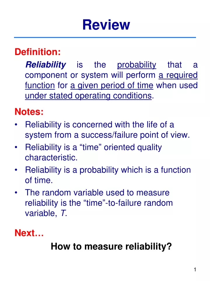
Review Definition: Reliability is the probability that a component or system will perform a required function for a given period of time when used under stated operating conditions. Notes: • Reliability is concerned with the life of a system from a success/failure point of view. • Reliability is a “time” oriented quality characteristic. • Reliability is a probability which is a function of time. • The random variable used to measure reliability is the “time”-to-failure random variable, T. Next… How to measure reliability?
Failure Distributions-- Reliability Measures Overview 1. Probability Functions Representing Reliability 1.1 Reliability Function 1.2 Cumulative Distribution Function (CDF) 1.3 Probability Density Function (PDF) 1.4 Hazard Function 1.5 Relationships Among R(t), F(t), f(t), and h(t) 2. Bathtub Curve -- How population of units age over time 3. Summary Statistics of Reliability 3.1 Expected Life (Mean time to failure) 3.2 Median Life and Bα Life 3.3 Mode 3.4 Variance
Probability Functions Representing Reliability • Reliability Function • Cumulative Distribution Function (CDF) • Probability Density Function (PDF) • Hazard Function • Relationships Among R(t), F(t), f(t), and h(t)
Reliability Function Definition: Reliability function is the probability that an item is functioning at any time t. Let T = “time”-to-failure random variable, reliability at time t is For example, reliability at time t=100s is R(100) = P(T >= 100) Properties:
Reliability Function Two interpretations: • R(t) is the probability that an individual item is functioning at time t • R(t) is the expected fraction of the population that is functioning at time t for a large population of items. Other names: • Survivor Function -- Biostatistics • Complementary CDF
CDF and PDF Cumulative Distribution Function, F(t) F(t)= P(T<t) =1-R(t) • Properties: • Interpretation: F(t) is the probability that an item fails before time t. Probability Density Function, f(t) • Properties: • Interpretation: f(t) indicates the likelihood of failure for any t, and it describes the shape of the failure distribution.
P(T>=t) P(T<t) T t Relationships Among R(t), F(t), and f(t)
Examples Example 1 Consider the pdf for the uniform random variable given below: where t is time-to-failure in hours. Draw the pdf, cdf and the reliability function. Solution f(t) pdf 1/100 T 100 f(t) Cdf & R(t) 1/100 100
Examples Example 2 Given the probability density function where t is time-to-failure in hours and the pdf is shown below: Graph the cdf and the reliability function. Solution
Examples Example 3 For the reliability function where t is time-to-failure in hours. • What is the 200 hr reliability? • What is the 500 hr reliability? • If this item has been working for 200 hrs, What is the reliability of 500 hrs? Solution
Examples Example 4 Given the following time to failure probability density function (pdf): where t is time-to-failure in hours. What is the reliability function? Solution
Examples Example 5 Given the cumulative distribution function (cdf): where t is time-to-failure in hours. • What is the reliability function? • What is the probability that a device will survive for 70 hr?
Hazard Function Motivation for Hazard Function It is often more meaningful to normalize with respect to the reliability at time t, since this indicates the failure rate for those surviving units. If we add R(t) to the denominator, we have the hazard function or “instantaneous” failure rate function as
Hazard Function Notes: • For small Δt values, which is the conditional probability of failure in the time interval from t to t+ Δt given that the system has survived to time t.
Hazard Function Notes (cont.): • The shape of the hazard function indicates how population of units is aging over time • Constant Failure Rate (CFR) • Increasing Failure Rate (IFR) • Decreasing Failure Rate (DFR) • Some reliability engineers think of modeling in terms of h(t) Other Names for Hazard Function • Reliability: hazard function/hazard rate/failure rate • Actuarial science: force of mortality/force of decrement • Vital statistics: age-specific death rate
Hazard Function Various Shapes of Hazard Functions and Their Applications
Plots of R(t), F(t), f(t), h(t)for the normal distribution R(t) f(t) F(t) h(t)
Relationships Among R(t), F(t), f(t), and h(t) One-to-One Relationships Between Various Functions Notes: The matrix shows that any of the three other probability functions (given by the columns) can by found if one of the functions (given by the rows) is known.
Examples Example 6 Consider the pdf used in Example 2 given by Calculate the hazard function. Solution
Examples Example 7 Given h(t)=18t, find R(t), F(t), and f(t). Solution
Bathtub Curve The failure of a population of fielded products is due to • Problems due to inherent design weakness. • The manufacturing and quality control related problems. • The variability due to the customer usage. • The maintenance policies actually practiced by the customer and improper use or abuse of the product.
Bathtub Curve Over many years, and across a wide variety of mechanical and electronic components and systems, people have calculated empirical population failure rates as units age over time and repeatedly obtained a bathtub shape: • Infant mortality (burn-in) period:decreasing failure rate early in the life cycle • Constant failure rate (useful life) period: nearly constant failure rate • Wear-out period: the failure rate begins to increase as materials wear out and degradation failures occur at an ever increasing rate.
Annual Rate of Accidents Young drivers Seniors 16-19 20-24 25-29 60-64 65-69 70-74 … Age Bathtub Curve An Example: Accident Rates and Age
Bathtub Curve Typical information for components of a PC
Summary Statistics of Reliability • Expected Life (Mean time to failure) • Median Life and BαLife • Mode • Variance
Expected Life E[T] is also called: • Mean Time to Failure (MTTF) for nonrepairable items • Mean Time between Failure (MTBF) for repairable items that can be completely renewed by repair E[T] is a measure of the central tendency or average value of the failure distribution, and it is known as the center of gravity in physics.
Expected Life Relationship between E[T] and R(t): • Show that E(T) can be re-expressed as • Sometimes, one expression is easier to integrate than the other exponential example, how?
Examples Example 8 Given that What is the MTTF? Solution
Median Life and Bα Life The median life, B50, divides the distribution into two equal halves, with 50% of the failure occurring before and after B50. Bα Life is the time by which α percent of the items fail. For example, B10life can be calculated by
Mode and Variance Modeis the time value at which the probability density function achieves a maximum. Mode is the most likely observed failure time. Variance
Examples Example 9 Consider the pdf used in Example 2 (triangle distribution) given by Calculate the MTTF, the B50 life (the median life), and the mode.
Examples Example 10 For the exponential distribution with mean=100, calculate the B50 life (the median life), and the mode.