Regression Diagnostics

Regression Diagnostics Using Residual Plots in SAS to Determine the Appropriateness of the Model

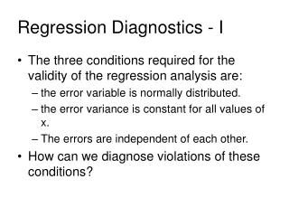
Introduction When conducting linear regression, it is important to make sure the assumptions (L.I.N.E.) behind the model are met. It is also important to verify that the estimated linear regression model is a good fit for the data (often a linear regression line can be estimated by SAS, even if it’s not appropriate—in this case it is up to you to judge whether the model is a good one).

Consider the Following Data Set: Peak blood level data (in mg/ml) were obtained for 20 patients for a single dose of a drug. In addition to the blood level, the patient’s weight (in lbs) and the amount of drug (in mg) were recorded. The data can be found in the file blood.txt with level (column 1), dose (column 2), and weight (column 3). Use the INFILE statement to read this data set into SAS: http://www.biostat.umn.edu/~susant/PH6415DATA/blood.txt

After you have checked your Log for any errors and the data set has been printed in the Output, so you can see there is no missing data, create a plot of the data to determine whether a linear relationship between level and weight seems justified:

Plot of Level * Weight

It appears from the plot that a linear relationship between blood level and weight may not be justified. There may be a slightly negative relationship between the two variables, but in general there does not appear to be a linear relationship. However, we will continue with linear regression (knowing that it may be inappropriate), in order to explore regression diagnostics.

PROG REG Submit the following program in SAS. In addition to the first two statements with which you are familiar, the third statement requests a plot of the residuals by weight and the fourth statement requests a plot of the studentized (standardized) residuals by weight:

Regression Output

Interpreting Output Notice that the overall F-test has a p-value of 0.2160, which is greater than 0.05. Therefore, we would conclude that blood level and weight are independent (fail to reject Ho: β1 = 0). Now look at the following plots:

Plot of Regression Line: Notice it is the same plot as the one you created from PROC GPLOT, except the fitted regression line has been added to it.

Plot of residuals * weight: you want an even spread of points above and below the dashed line. This is a good way to eyeball the data for potential outliers.

Plot of studentized residuals * weight: look for values with an absolute value larger than 2.6 to determine if there are any outliers.

You can see from the plot that the observation with weight = 128 (observation #4) is an outlier. The residual plots also help you determine whether the assumption of constant variance is met. Because the residuals appear to be randomly scattered without any definite pattern, this suggests that the data are independent with constant variance.

The Normality Assumption A convenient way to test for normality is by constructing a “Normal Quantile Quantile” plot. This plots the residuals you would see under normality versus the residuals that are actually observed. If the data are completely normal, the residuals will follow a 45° line. Use the following code in SAS to make the NQQ plot: PLOTresidual. * nqq.; RUN;

Residual vs. NQQ Plot

Interpreting the NQQ Plot The residuals do not clearly follow a 45° line. Because the tails of this line seem curved, this suggests that the data may be skewed, not normally distributed.

Conclusions When conducting linear regression, it is important to verify whether the assumptions under which the model is created (L.I.N.E.) are met. This tutorial has given you an introduction to ways of assessing whether your data meets the criteria.

Regression Diagnostics