Limits and the Law of Large Numbers

Limits and the Law of Large Numbers Lecture XIV

Almost Sure Convergence • Let w represent the entire random sequence {Zt}. As discussed last time, our interest typically centers around the averages of this sequence:

Definition 2.9: Let {bn(w)} be a sequence of real-valued random variables. We say that bn(w) converges almost surely to b, written if and only if there exists a real number b such that

The probability measure P describes the distribution of w and determines the joint distribution function for the entire sequence {Zt}. • Other common terminology is that bn(w) converges to b with probability 1 (w.p.1) or that bn(w) is strongly consistent for b.

Example 2.10: Let where {Zt} is a sequence of independently and identically distributed (i.i.d.) random variables with E(Zt)=m<. Then by the Komolgorov strong law of large numbers (Theorem 3.1).

Proposition 2.11: Given g: RkRl (k,l<∞) and any sequence {bn} such that where bn and b are k x 1 vectors, if g is continuous at b, then

Theorem 2.12: Suppose • y=Xb0+e; • X’e/na.s. 0; • X’X/a.s.M, finite and positive definite. • Then bn exists a.s. for all n sufficiently large, and bna.s.b0.

Proof: Since X’X/na.s.M, it follows from Proposition 2.11 that det(X’X/n) a.s.det(M). Because M is positive definite by (iii), det(M)>0. It follows that det(X’X/n)>0 a.s. for all n sufficiently large, so (X’X/n)-1 exists a.s. for all n sufficiently large. Hence

In addition, • It follows from Proposition 2.11 that

Convergence in Probability • A weaker stochastic convergence concept is that of convergence in probability. • Definition 2.23: Let {bn(w)} be a sequence of real-valued random variables. If there exists a real number b such that for every e > 0, as n, then bn(w) converges in probability to b.

The almost sure measure of probability takes into account the joint distribution of the entire sequence {Zt}, but with convergence in probability, we only need to be concerned with the joint distribution of those elements that appear in bn(w). • Convergence in probability is also referred to as weak consistency.

Theorem 2.24: Let { bn(w)} be a sequence of random variables. If If bn converges in probability to b, then there exists a subsequence {bnj} such that

Convergence in the rth Mean • Definition 2.37: Let {bn(w)} be a sequence of real-valued random variables. If there exists a real number b such that as n for some r > 0, then bn(w) converges in the rth mean to b, written as

Proposition 2.38: (Jensen’s inequality) Let g: R1R1 be a convex function on an interval B R1 and let Z be a random variable such that P[ZB]=1. Then g(E(Z)) E(g(Z)). If g is concave on B, then g(E(Z))E(g(Z)).

Proposition 2.41: (Generalized Chebyshev Inequality) Let Z be a random variable such that E|Z|r < , r > 0. Then for ever e > 0

Theorem 2.42: If bn(w)r.m. b for some r > 0, then bn(w)p b.

Laws of Large Numbers • Proposition 3.0: Given restrictions on the dependence, heterogeneity, and moments of a sequence of random variables {Zt}, where

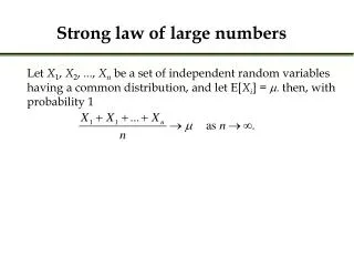
Independent and Identically Distributed Observations • Theorem 3.1: (Komolgorov) Let {Zt} be a sequence of i.i.d. random variables. Then if and only if E|Zt| <  and E(Zt) = m. • This result is consistent with Theorem 6.2.1 (Khinchine) Let {Xi} be independent and identically distributed (i.i.d.) with E[Xi] = m. Then

Proposition 3.4: (Holder’s Inequality) If p > 1 and 1/p+1/q=1 and if E|Y|p <  and E|Z|q < , then E|YZ|[E|Y|p]1/p[E|Z|q]1/q. • If p=q=2, we have the Cauchy-Schwartz inequality

Asymptotic Normality • Under the traditional assumptions of the linear model (fixed regressors and normally distributed error terms) bn is distributed multivariate normal with: for any sample size n.

However, when the sample size becomes large the distribution of bn is approximately normal under some general conditions.

Definition 4.1: Let {bn} be a sequence of random finite-dimensional vectors with joint distribution functions {Fn}. If Fn(z) F(z) as n for every continuity point z, where F is the distribution function of a random variable Z, then bnconverges in distribution to the random variable Z, denoted

Other ways of stating this concept are that bnconverges in law to Z: Or, bn is asymptotically distributed asF In this case, F is called the limiting distribution of bn.

Example 4.3: Let {Zt} be a i.i.d. sequence of random variables with mean m and variance s2 < . Define Then by the Lindeberg-Levy central limit theorem (Theorem 6.2.2),

Theorem (6.2.2): (Lindeberg-Levy) Let {Xi} be i.i.d. with E[Xi]=m and V(Xi)=s2. Then ZnN(0,1). • Definition 4.8: Let Z be a k x 1 random vector with distribution function F. The characteristic function of Z is defined as where i2=-1 and l is a k x 1 real vector.

Example 4.10: Let Z~N(m,s2). Then • This proof follows from the derivation of the moment generating function in Lecture VII.

Specifically, note the similarity between the definition of the moment generating function and the characteristic function: • Theorem 4.11 (Uniqueness Theorem) Two distribution functions are identical if and only if their characteristic functions are identical.

Note that we have a similar theorem for moment generating functions. • Proof of Lindeberg-Levy: • First define f(l) as the characteristic function for Zt-m and let fn(l) be the characteristic function of

By the structure of the characteristic function we have

Taking a second order Taylor series expansion of f(l) around l=0 gives Thus,

Thus, by the Uniqueness Theorem the characteristic function of the sample approaches the characteristic function of the standard normal.

Limits and the Law of Large Numbers