Download
1 / 43
430 likes | 434 Views
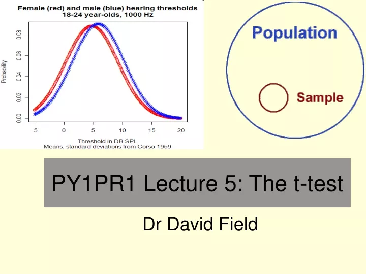
PY1PR1 Lecture 5: The t-test. Dr David Field. Summary. Andy Field, 3 rd Edition, chapter 9 covers today's lecture But one sample t and formulas are not covered The t test for independent samples Comparing the means of two samples of subjects Degrees of freedom

E N D
PY1PR1 Lecture 5: The t-test Dr David Field
Summary • Andy Field, 3rd Edition, chapter 9 covers today's lecture • But one sample t and formulas are not covered • The t test for independent samples • Comparing the means of two samples of subjects • Degrees of freedom • The paired samples t test (also known as repeated measures and related samples) • Comparing the means of two experimental conditions when the same sample participated in both conditions • The one sample t test • Comparing the mean of a single sample against a fixed value, e.g. 50% chance performance, or 0 • Effect size • The degree to which changes in a DV are caused by the IV relative to other sources of variation • 95% confidence interval of the difference between sample means
The story so far…. • In workshop 3 you produced an error bar chart for the blueberries versus sugar cubes with exam scores experiment • The 95% confidence intervals around the two means overlapped, so we could not be sure that the two samples were from different populations • We could not reject the null hypothesis • We could not be sure that we have failed to reject the null hypothesis • Today, we will use the t test to make a direct test of the null hypothesis for that experiment • By performing a t test you arrive at a significance level or p value, which is the probability of obtaining the difference between the means of experimental conditions by random sampling from a null distribution
The t statistic 9.3 9.3.1 • There are several variations on how t is calculated that depend on the type of experiment (independent samples, repeated measures, one sample) • But these are variations on a general theme • Higher values of t reflect greater statistical significance Difference between two means Variation in data
In the following examples the difference between the means is the same in all three cases • But the variability of the samples is different t will be smaller than ‘medium’ t will be larger than ‘medium’
The t statistic • The size of t can be increased in three ways • increase the difference between the two sample means • reduce the variability in the two samples • Increase the number of participants Difference between two means Variation in data
In different types of experiment different methods are used to calculate the SE of the difference The t statistic • There are several variations on how t is calculated that depend on the type of experiment (independent samples, repeated measures, one sample) • But these are variations on a general theme mean sample 1 – mean sample 2 SE of the difference
SE of the difference (see lecture 4) • The SE of the difference is similar to the SE of a sample mean • It reflects an underlying sampling distribution of many possible repetitions of the experiment using that exact sample size, where in each case the difference obtained between the means would be slightly different • The key thing is that the SE gets smaller as the sample size increases and as the underlying SD of the population of interest reduces • Because the t formula involves dividing by the SE of the difference t is in units of SE • just as Z scores are in units of SD mean sample 1 – mean sample 2 SE of the difference
SE of the difference for independent samples • Independent samples (or between subjects) is where separate samples of participants are tested in each experimental condition • We will use the effects of eating blueberries versus sugar cubes on exam scores as an illustration • In this case the SE of the difference has to take into account the fact that there are two samples contributing to the part of the unsystematic variation in the scores that is not due to the IV • IQ and hours studied are things the researchers are not interested in that might contribute to the variability of scores in both samples of the blueberry experiment
SE of the difference for independent samples • N is the number of participants in the groups, which may be unequal • Recall that the variance is the sum of squared differences from the mean divided by N-1 (see lecture 1) • This formula is very similar to that used in the z test (lecture 4). • But the way that t is converted to a p value is slightly different from the way z is converted to a p value Sample 2 variance Sample 1 variance N sample 2 N sample 1
t formula for independent samples 9.5 Sample 2 mean Sample 1 mean t = Sample 2 variance Sample 1 variance N sample 2 N sample 1
Blueberry experiment example 50.77 57.47 t = 94.8 106.8 30 30 t = 2.58
Converting t to a p value (significance level) • The t statistic is a measure of the difference between the sample means in units of SE (i.e. units of estimated measurement error) • It is a measure of how big the effect of the IV is compared to unsystematic variation • random allocation of participants to conditions helps to insure that other sources of variation do not co-vary with the IV • Two sample means will differ even under the null hypothesis, where the only source of variation in the data is unsystematic • what is the probability of a a value of t this big or bigger arising under the null hypothesis?
What differs from the z test? • For the z test, the obtained value of z is referred to the standard normal distribution, and the proportion of the area under the curve with that value of z or greater is the p value • However, when sample sizes are small the standard normal distribution is actually a bad model of the null distribution • it’s tails are too thin and values close to the mean are too common • The t distribution has much fatter tails, accurately representing the chances of large differences between sample means occurring by chance when samples are small • Unlike the standard normal distribution, the t distribution changes shape as the sample size increases • As N increases the tails get thinner, and if N > 30, it is almost identical to the z distribution
The standard normal distribution compared to the t distribution when N = 2 Blue is the standard normal distribution Red is the t probability distribution if N = 2 in both groups The proportion of area under the curve that is, e.g., > 2 is much greater for the t distribution The proportion is 14.7% for t and 2.3% for z
The standard normal distribution compared to the t distribution when N = 4 Blue is the standard normal distribution Red is the t probability distribution if N = 4 both groups The proportion of area under the curve that is, e.g., > 2 is now reduced for the t distribution The proportion is 5.0% for t and 2.3% for z
Degrees of Freedom (DOF) Jane Superbrain 2.2 • The shape of the t distribution under the null hypothesis changes as sample size (N) goes up • This is because the number of degrees of freedom increases as the two sample sizes go up • and the shape of the t distribution is directly specified by the DOF, not N • The degrees of freedom for the independent samples t test are given by (group one sample size - 1) + (group two sample size -1) • All statistics have degrees of freedom, and for some statistics the formula for working them out is more complicated • Fortunately, SPSS calculates DOF for you
Degrees of freedom (DOF) • The DOF are the number of elements in a calculation that are free to vary. • If you know only that four numbers have a mean of 10 you can say nothing about what the four numbers might be • But if you also know that the first three numbers are 8, 9, and 11 • Then the fourth number must be 12 • If you only know that the first two numbers are 8 and 9 there are still an infinite possible number that the third and fourth numbers can take • Therefore, this calculation has 3 DOF
Converting t to a p value (significance level) • Having worked out the value of t and the number of DOF associated with the calculation of t, SPSS will report the exact probability(p value) of obtaining that value of t under the null hypothesis that both samples were selected randomly from populations with identical means • The p value is equal to the proportion of the area under the curve of the appropriate t distribution where the values are as big or bigger than the obtained value of t • In the past you had to look up the p value yourself in statistical tables of DOF versus t at the back of a textbook….. • Remember that if p < 0.05 you can reject the null hypothesis and say that the effect of the IV on the DV was statistically significant
Blueberry example • In the blueberry experiment there was a difference of 6.7% in the predicted direction, but the 95% confidence intervals around the means of the two groups overlapped, so it is useful to perform the t test to see if there is enough evidence to reject the null hypothesis • “The effect of supplementing diet with blueberries compared to sugar cubes on exam scores was statistically significant, t(58) = 2.58, p = 0.006 (one tailed).” • This is an incomplete example of reporting experimental results • A full example will be given later • We write (one tailed) and divide the p value SPSS gives by 2 because the researchers predicted that blueberries would improve exam scores, rather than just changing them • t is sometimes negative, but this has no special meaning, it just depends which way round you enter the variables in the t test dialogue box in SPSS
Related t-test 9.6 • This is also known as paired samples or repeated measures • Use it when the same sample of participants perform in both the experimental and control conditions • For example, if you are interested in whether reaction times differ in the morning and the afternoon, it would be more efficient to use the same sample for both measurements • If you suspect that practice (or fatigue) effects will occur when the DV is measured twice in the same person then counterbalance the order of testing to prevent order effects from being confounded with the IV • In the example you’d test half the participants in the morning first and then in the afternoon, and the other half would be tested in the afternoon first and then in the morning • Order effects will then contribute only to unsystematic variation
Advantages of related t over independent t • In the blueberry experiment, there was variation in scores in each group due to IQ and hours studied. • this variation was included in the SE part of the equation • If you tested the same participants twice, once in the blueberry condition, and once in the sugar cube condition, employing two equally difficult exams, then IQ scores and study habits would be equalised across the two experimental conditions • This would reduce the risk of a type 1 error occurring due to chance (sampling) differences in unsystematic variation between conditions • It would no longer be possible, by chance, for the majority of the higher IQ and hard working participants to end up in one of the two experimental conditions • If you constructed the experiment in this repeated measures way, and used the independent samples t formula this would already be an improvement on the separate samples design • But, a bigger improvement in the sensitivity of the experiment can be achieved by changing how the SE is calculated
Advantages of related t over independent t • In the repeated measures design, each score can be directly paired (compared) with a score in the other experimental condition • We can see that John scored 48 in the exam when supplemented with sugar cubes and 52 when he ate blueberries • There was no meaningful way to compare the score of an individual participant with any other individual in the other condition when independent samples were used • In the repeated measures case we can calculate a difference score for John, which is 4 • If Jane scored 70 (sugar cubes) and 72 (blueberries) then her difference score is 2 • Jane has a very different overall level of performance compared to John, but we can ignore this, and calculate the error term using only the difference scores • In the independent samples t the massive difference between John and Jane had to be included in the error term
x x x x x Data table for independent samples t test
t formula for related samples Mean difference between conditions t = SD of the difference Sample size (Compare independent samples t) Sample 2 mean Sample 1 mean t = Sample 2 variance Sample 1 variance N sample 2 N sample 1
Worked example of related t • The SD of the difference scores is 0.061 sec and N is 5 • Therefore, SE is 0.061 / square root of 5 • 0.061 / 2.23 = 0.027 • t = Mean dif / SE • -0.10 / 0.027 • t = -3.65
Converting related t to a p value • The null hypothesis is that the mean difference between the two conditions in the population is zero • DOF are given by sample size – 1 for related t • DOF are needed to determine the exact shape of the probability distribution, in exactly the same way as for independent samples t • The value of t is referred to the t distribution, and the p value is the proportion of the area under the curve equal to or greater than the obtained t • This is the probability of a mean difference that big occurring by chance in a sample if the difference in the population was zero • The repeated t test is reported in the same way as the independent t test
Reaction time example • “It took longer to respond in the morning than in the afternoon, t(4) = -3.65, p = 0.02 (two tailed).” • This is an incomplete example of reporting experimental results • A full example will be given later • This is a two tailed test because the researchers thought that circadian rhythms would result in a different rtm in the afternoon, but they were not able to predict the direction of the difference in advance • For a two tailed test you have to consider both tails of the probability distribution, in this case the area under the curve that is greater than 3.65 and less than -3.65 • SPSS does this by default
One sample t-test • Sometimes, you want to test the null hypothesis that the mean of a single sample is equal to a specific value • For example, we might hypothesize that, on average, students drink more alcohol than the people of similar age in the general population • Imagine that a previous study used a large and appropriately selected sample to establish that the mean alcohol consumption per week for UK adults between the ages of 18 and 22 is 15 units • We can make use of their large and expensive sample, which provides a very good estimate of the population mean • To test the hypothesis we could randomly select a single sample of students aged 18-22 and compare their alcohol consumption with that from the published study • The null hypothesis will be that the mean units of alcohol consumed per week in the student sample is 15
This is the SE of the sample mean (Compare related samples t formula) Mean difference between conditions t = SD of the difference Sample size One sample t formula Mean difference from null hypothesis t = SD of the sample Sample size
Worked example of one sample t • The SD of the difference scores is 4.14 units and N is 5 • Therefore, SE is 4.41 / square root of 5 • 4.41 / 2.23 = 1.85 • t = Mean dif / SE • 0.2 / 1.85 • t = 0.107
Converting one sample t to a p value • The null hypothesis is that the population mean is the same as the fixed test value (15 in this case) • DOF are given by sample size – 1 • DOF are needed to determine the exact shape of the probability distribution, in exactly the same way as for independent samples t • The value of t is referred to the t distribution, and the p value is the proportion of the area under the curve equal to or greater than the obtained t • This is the probability of the sample mean being that different from the fixed test value if the true population mean is equal to the fixed test value
Alcohol consumption example • “We found no evidence that students consume more alcohol than other people in their age group, t(4) = 0.10, p > 0.05, NS” • This is an incomplete example of reporting experimental results • A full example will be given later • NS is short for for non-significant • The results of a t test are non significant if p is larger than 0.05 (5%).
Effect size (Cohen’s d ) • Statistical significance (i.e. p of data under null hypothesis of < 0.05) is not equivalent to scientific importance • If SPSS gives a p value of 0.003 for one t test, and 0.03 for another t test, then the former is “statistically highly significant” but it is NOT a “bigger effect” or “more important" than the latter • This is because the SE of the difference depends partly on sample size and partly on the SD of the underlying population (as well as on the size of the mean difference) • If the sample size it large a trivially small difference between the means can be statistically highly significant • If the two underlying populations of scores in an independent samples t test have a small SD then a trivially small difference in means will again be statistically highly significant
Effect size (Cohen’s d ) • For these reasons it is becoming increasingly common to report effect size alongside a null hypothesis test Condition 1 mean – Condition 2 mean d = SD Condition 1 + SD condition 2 2 • The key difference from the t formula is that sample size is not part of the formula for d • like z scores, d is expressed in units of SD • Effect size is basically a z score of the difference • SPSS does not report effect size as part of the t test output, but you can easily calculate it yourself
Effect size in the blueberry example • d is 6.7 / 10.05 = 0.66 • This means the mean difference of 6.7% between the two groups is equal to 0.66 pooled SD blue 57.47% – sugar 50.77% d = Blue SD 10.3% + sugar SD 9.7% 2
Interpreting effect size • Cohen (1988) • d 0.2 is a small effect • d 0.5 is a medium effect • d 0.8 is a large effect • d of > approx 1.5 is a very large effect • Warning: Andy Field 3rd Edition uses a different measure of effect size, called r • For this course, you must use Cohen’s d
95% confidence interval of the difference 9.4.5 • Previously, you calculated a 95% confidence interval around a sample mean, and it is also possible to calculate a 95% confidence interval of the difference between two sample means • In the blueberry example, the difference in exam scores between the two groups was 6.7% • This difference is actually a point estimate produced by a single experiment, and in principle there is an underlying sampling distribution of similar experiments with the same sample size • Each time you repeated the experiment the result (mean difference) would be slightly different • The point estimate of the difference can be converted to an interval estimate using a similar method to that for calculation of an interval estimate based on a sample mean
95% confidence interval of the difference • For the blueberry example, SPSS reports a 95% confidence interval of 1.5 to 11.9 for the underlying mean difference in the population • This means that if we replicated the experiment with the same sample sizes in the sugar and blueberry groups we could be 95% confident of observing a difference in exam scores of somewhere between 1.5 and 11.9 percentage points • Reporting the 95% confidence interval of the difference is becoming common practice in journal articles
Reporting t test results • Here is an example of how to put all the different statistics from today’s lecture into a paragraph • “Participants in the blueberry condition achieved higher exam scores (mean = 57.47%, SD = 10.3%) than those in the sugar cube condition (mean = 50.77%, SD = 9.7%). The mean difference between conditions was 6.7%, which is a medium effect size (d = 0.66); the 95% confidence interval for the estimated population mean difference is between 1.5 and 11.9%. An independent t test revealed that, if the null hypothesis were true, such a result would be highly unlikely to have arisen (t(58) = 2.58; p = 0.006 (one tailed)).” • This paragraph gives the reader more useful information than the traditional practice of reporting only the null hypothesis test • Always report descriptive statistics (mean, SD, effect size, confidence interval of difference) before inferential statistics that test the hypothesis and have a p value (for example, t).
List of statistical terms for revision • t statistic • degrees of freedom (DF) • independent samples t test • related or paired samples t test • one sample t test • standard error of differences • effect size