Download
1 / 18
200 likes | 540 Views
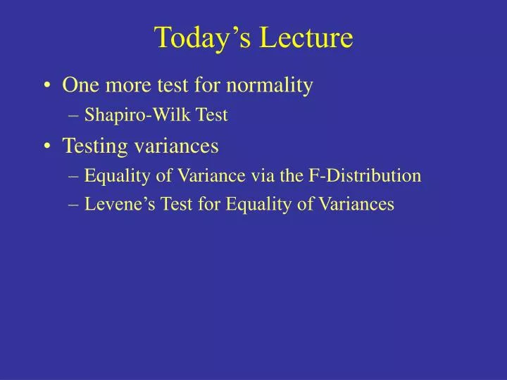
Today’s Lecture. One more test for normality Shapiro-Wilk Test Testing variances Equality of Variance via the F-Distribution Levene’s Test for Equality of Variances. Reference Material. Shapiro and Wilk, 1965. Biometrika (52:3 and 4) pgs. 591-611. Burt and Barber, page 325

E N D
Today’s Lecture • One more test for normality • Shapiro-Wilk Test • Testing variances • Equality of Variance via the F-Distribution • Levene’s Test for Equality of Variances
Reference Material • Shapiro and Wilk, 1965. Biometrika (52:3 and 4) pgs. 591-611. • Burt and Barber, page 325 • Levene, 1960. In Contributions to Probability and Statistics: Essays in Honor of Harold Hotelling, I. Olkin et al. eds., Stanford University Press, pp. 278-292.
More Pretests • The tests presented in today’s lecture are pretests that can help to verify the assumptions of a parametric hypothesis test • The first is one of the strongest tests for normality • The second is one of the simplest tests for determining if a pooled or non-pooled variance t-test is required • The last allows for a comparison of variances in a multiple category layout like the analysis of variance
Shapiro-Wilk • The Shapiro-Wilk is one of the strangest tests that I have encountered thus far in my statistical explorations • But it is either the best or the second best test of normality in existence • It excels at normality testing small samples and is the definitive test for n<30
Curiouser and Curiouser • A brief rundown of the strangeness associated with the Shapiro-Wilk • You fail reject the null when your observed value is greater than your critical value (that’s right, the critical region on this test is in the small tail) • The test actually pairs observations from within the sample to determine normality • The number of pairs is determined by nearly the same equation that you would use to determine the median
So How Does It Work? • The W-Statistic: • Recall that the variance of a sample is s2 • So really all we are required to give is the sum of the squared deviations from the mean (plus this term b2) • b2is a bit more complex, but it is more odd than difficult
Getting to B-Squared • The b term is actually a weighted comparison of all the pairs within the sample • The way that it works is that you sort all of your data from least to greatest • Then you create k number of pairs from the sample with k=n/2 if n is even and k=n+1/2 if n is odd (note that k is the median of the sample) • Each pair has a companion that is from the other end of the sample • Example: Given the following set of numbers- 1,2,3,4,5,100 your pairs would be as follows: • 100 and 1, 5 and 2, and 4 and 3
Once You Have Your Pairs • The pairs are important because you will be taking the difference between the large value and the small value (100-1=99, 5-2=3, 4-3=1) • Once you have all your differences, you then assign them weights (from a W-weight table • Once you have the weights, you multiply each one by its pair and then sum them all • This sum is b, which you then square
Strange, don’t you think? • Let’s go to Excel • But first let’s show you the equation for b The median Big and Little Pairs ai weight (from math that you don’t want to have to learn) – basically the weights are the result of an expected normal distribution and its resulting covariance matrix
Results • W=0.952165 • This isn’t very small, so we are going to fail to reject • H0: Normal HA: Not Normal (note the wording here, we are not saying that this test shows that the data is normal, we are only saying that it fails to show that the data is not normal) • W(critical) for 0.05 and n=20 is 0.905 • Note that this distribution is severely skewed so our result of 0.952 has a p-value of around 0.40 • This sample is suitable for parametric analysis
Shapiro-Wilk Tables Pair Coefficients (weights) Critical levels for significance
Equality of Variance via Ratio • Assumptions: • s12 and s22 are independent estimates of σ2 • The population from which the samples are drawn is normal (This means you had better check for normality first) • H0: σ12 = σ22 Ha: σi2 ≠ σj2 • Statistic: s12/s22 (I typically place the larger variance in the numerator of the equation, but it doesn’t matter for two tailed tests) • Once you compute the statistic you find the F-distribution in the appendix of your book (page 613) and then use n1-1 and n2-1 for your degrees of freedom
Example • A couple of weeks ago we used two samples in a t-test. The first sample had an n=12 and a variance of 17.3, the second sample had an n=10 and a variance of 18.9 • 18.9/17.3=1.092 • A look at our tables with 11 and 9 degrees of freedom at alpha=0.05 will tell us that a critical value of 3.96 (we have to use 10 for n1, because there is no 11 column) • Since 1.09<3.96, we fail to reject the null
Levene’s L-Statistic • Test for the equality of variance in multiple categories • H0: σ12 = σ22 = … = σk2 • Ha: σi2 ≠ σj2for at least one pair (i,j). • The statistic is run on the deviations from the mean but is very similar to the ANOVA in terms of computation • The test uses the F-distribution to determine significance
The Equation All data in each category is “differenced” by its category mean This is a categorical mean of differences This is the global mean of differences This is a sum of squares between, but on the xij differences dfb This is a sum of squares within, but on the xij differences dfw
Results • After all of our computations, we find an L value of 2.41 • Since our degrees of freedom are k-1=2 and N-k=12 an alpha of 0.05 would require a critical value for L of 3.88 • Since 2.41<3.88 we fail to reject the null of equal variances between categories • This data set is suitable for parametric analysis via an ANOVA
Homework • Given two data sets, test for normality using the Shapiro Wilk and then test for equality of variance via ratio. • Once you have completed both tests, recommend the correct test for comparing the samples. • Your choices are the T-Test (pooled variance), T-Test (non-pooled variance) and the Wilcoxon Rank-Sum Test