Download
1 / 50
500 likes | 502 Views
Hydrologic Properties of the Landscape. David G Tarboton Utah State University http://www.engineering.usu.edu/dtarb/ david.tarboton@usu.edu. Outline. Slope and Contributing Area The D Algorithm TOPMODEL Wetness Index Terrain Stability Mapping SINMAP ArcView Extension

E N D
Hydrologic Properties of the Landscape David G Tarboton Utah State University http://www.engineering.usu.edu/dtarb/ david.tarboton@usu.edu
Outline • Slope and Contributing Area • The D Algorithm • TOPMODEL Wetness Index • Terrain Stability Mapping SINMAP ArcView Extension • Topographic texture and drainage density • TARDEM programs for watershed and channel network delineation
? Topographic Slope Topographic Definition Drop/Distance Limitation imposed by 8 grid directions.
Stream line Contour line Upslope contributing area a Contributing Area Grid Based Evaluation Topographic Definition Specific catchment areaa is the upslope area per unit contour length [m2/m m]
The D Algorithm Tarboton, D. G., (1997), "A New Method for the Determination of Flow Directions and Contributing Areas in Grid Digital Elevation Models," Water Resources Research, 33(2): 309-319.) (http://www.engineering.usu.edu/cee/faculty/dtarb/dinf.pdf)
Contributing Area using D Contributing Area using D8
D Dw S Topmodel - Assumptions • The soil profile at each point has a finite capacity to transport water laterally downslope. e.g. or
D Dw S Topmodel - Assumptions Specific catchment areaa [m2/m m] (per unit coutour length) • The actual lateral discharge is proportional to specific catchment area. • R is • Proportionality constant • may be interpreted as “steady state” recharge rate, or “steady state” per unit area contribution to baseflow.
D Dw S Topmodel - Assumptions Specific catchment areaa [m2/m m] (per unit coutour length) • Relative wetness at a point and depth to water table is determined by comparing qact and qcap • Saturation when w > 1. i.e.
D Dw S Topmodel Specific catchment areaa [m2/m m] (per unit coutour length) z
Slope Specific Catchment Area Wetness Index ln(a/S) from Map Calculator. Average, l = 6.91
Numerical Example T=2 m2/hr • K=10 m/hr • f=5 m-1 • R=0.0002 m/hr • l=6.91 Map calculator -( [ln(sca/S)] - 6.91)/5+0.46
SINMAP - Terrain Stability Mapping Arcview ExtensionR T Pack, D G Tarboton, C.N. Goodwin • Illustrates GIS as a spatial modeling environment • Illustrates tight integration of model into GIS • Utilizes GRIDIO application programmers interface to access Grids from external programs • Utilizes customizability of ArcView to provide easy to use interface
Where is it Used • Forest and watershed management, forestry and forest engineering. • Determine volume of harvestable timber in annual allowable cut calculations. • Better plan timber development to minimize occurrence of landslides and resulting impacts.
Theoretical Basis • The infinite plane slope stability model with wetness (pore pressure) obtained from a topographically based steady state hydrology model has been used to map terrain stability (e.g. Montgomery and Dietrich, 1994, WRR p1153) Stream line Contour line Stream tube Upslope contributing area a 1. Relative Wetness h q 2. Dimensionless Cohesion Density Ratio (assumed a constant of 0.5)
Area-Slope Plot FS > 1 w = 1 Stable, Saturated FS < 1 Unstable FS > 1 w < 1 Stable, Unsaturated
But • Soil parameters, C, f, T are uncertain and spatially variable. • Recharge parameter R is spatially and temporally variable. range P • Define Stability Index • SI = Prob(FS > 1) C1 C2
Most conservative parameter limits Most destabilizing parameter limits FS < 1 for all possible parameters SI = 0 SI = Prob(FS >1) FS* > 1 SI = FS* *(using most conservative end of each parameter range) Area-Slope plot with uncertainty
SI derived analytically for each region e.g. for region 2
SINMAP Inputs • Topography (dictated by DEM) • a - specific catchment area • θ - slope angle • Soil Parameters (given as a range) • C - dimensionless cohesion • tan Φ- tan of soil internal friction angle • R/T - soil hydraulic parameter
1. Specific Catchment Area Map 2. Stability Index Map 3. Soil Wetness Map 4. Calibration Plot 5. Statistical Tables SINMAP Outputs
SINMAP Implementation Spatial Analyst includes aC programming API (Application Programming Interface)that allows you toread and write ESRI grid data sets directly. Excerpt from gioapi.h / * GetWindowCell - Get a cell within the window for a layer, * Client must interpret the type of the output 32 Bit Ptr * to be the type of the layer being read from. * * GetWindowCellFloat - Get a cell within the window for a layer as a 32 Bit Float * * GetWindowCellInt - Get a cell within the window for a layer as a 32 Bit Integer * * PutWindowCell - Put a cell within the window for a layer. * Client must ensure that the type of the input 32 Bit Ptr * is the type of the layer being read from. * * PutWindowCellFloat - Put a cell within the window for a layer as a 32 Bit Float * * PutWindowCellInt - Put a cell within the window for a layer as a 32 Bit Integer */ int GetWindowCell(int channel, int rescol, int resrow, CELLTYPE *cell); int GetWindowCellFloat(int channel, int rescol, int resrow, float *cell); int GetWindowCellInt(int channel, int rescol, int resrow, int *cell); int PutWindowCellFloat(int channel, int col, int row, double fcell); int PutWindowCellInt(int channel, int col, int row, int icell); int PutWindowCell(int channel, int col, int row, CELLTYPE cell);
' SINMAP.c.area ' BaseName is the full directory path name of the input DEM grid BaseName = Self.Get(0) 'get the procedure from the dll library area = DLLProc.Make(_avlsmDLL,"area",#DLLPROC_TYPE_INT16, {#DLLPROC_TYPE_STR,#DLLPROC_TYPE_STR,#DLLPROC_TYPE_INT32, #DLLPROC_TYPE_INT32}) if (area = NIL) then av.Run("SINMAP.Error.OpFail",{2}) end error = area.Call({BaseName+"ang",BaseName+"sca", 0, 0}) if (error > 0) then av.Run("SINMAP.Error.OpFail",{"Grid and/or memory error reading/writing in area.c"}) end
Examples of differently textured topography Badlands in Death Valley.from Easterbrook, 1993, p 140. Coos Bay, Oregon Coast Range. from W. E. Dietrich
Canyon Creek, Trinity Alps, Northern California. Photo D K Hagans
Gently Sloping Convex Landscape From W. E. Dietrich
Topographic Texture and Drainage Density Same scale, 20 m contour interval Driftwood, PA Sunland, CA
Channel network delineation options 4 3 2 1 1 1 1 1 5 6 7 1 1 4 3 3 1 8 1 2 1 1 12 1 1 1 2 16 2 1 3 6 25 Accumulation Area
100 grid cell constant support area threshold stream delineation
200 grid cell constant support area based stream delineation
Channel network delineation options 4 3 2 1 1 1 1 1 1 1 1 1 1 5 6 7 1 1 1 4 2 3 2 2 3 1 1 Grid Order 8 1 1 1 2 1 1 1 1 3 12 1 1 1 1 1 1 2 1 16 3 1 2 1 1 2 3 6 2 25 3 Accumulation Area
Local Curvature Computation(Peuker and Douglas, 1975, Comput. Graphics Image Proc. 4:375) 43 48 48 51 51 56 41 47 47 54 54 58
TARDEM Components • Grid Processing • Flood • D8 • Dinf • Aread8 • Areadinf • Gridnet • Grid to Hierarchical Vector Network • Netsetup • Hierarchical Vector to Arc Coverage • Arclinks • Arcstreams • Network and Subwatershed Analysis • Linkan • Streaman • Asfgrid • Subbasinsetup
AREA 2 3 AREA 1 12 Questions and Demo?