Download
1 / 44
440 likes | 590 Views
CS 326 A: Motion Planning. http://robotics.stanford.edu/~latombe/cs326/2002 Radiosurgical Planning. Radiosurgery. Minimally invasive procedure that uses an intense, focused beam of radiation as an ablative surgical instrument to destroy tumors. Tumor = bad. Critical structures

E N D
CS 326 A: Motion Planning http://robotics.stanford.edu/~latombe/cs326/2002 Radiosurgical Planning
Radiosurgery Minimally invasive procedure that uses an intense, focused beam of radiation as an ablative surgical instrument to destroy tumors Tumor = bad Critical structures = good and sensitive Brain = good
The Radiosurgery Problem Dose from multiple beams is additive
Tumor Critical Treatment Planning for Radiosurgery • Determine a set of beam configurations that will destroy a tumor by cross-firing at it • Constraints: • Desired dose distribution • Physical properties of the radiation beam • Constraints of the device delivering the radiation • Duration/fractionation of treatment
Conventional Radiosurgical Systems • Isocenter-based treatments • Stereotactic frame required Gamma Knife LINAC System Luxton et al., 1993 Winston and Lutz, 1988
“Cold Spots” where coverage is poor • “Hot Spots” where the spheres overlap • Over-irradiation of healthy tissue Isocenter-Based Treatments Nonspherically shaped tumors are approximated by multiple spheres • All beams converge at the isocenter • The resulting region of high dose is spherical
Stereotactic Frame for Localization • Painful • Fractionation of treatments is difficult • Treatment of extracranial tumors is impossible
Optimization Approach to Planning • Treatment planning variables: • Isocenter locations • Treatment arcs • Collimator diameter • Beam weights • User specifies most planning variables • User defines constraints on dose to points and optimization function • Optimization technique determines beam weights [Bahr, 1968; Langer et al. 1987; Webb, 1992; Carol et al., 1992; Xing et al., 1998, …]
Motion-Planning Approach • Configuration space of the beam is a unit sphere • Construct free space by projecting critical structures onto the sphere • Search for longest arcs in free space Critical Structure Construction of free space [Schweikard, Adler, and Latombe, 1992, 1993]
The CyberKnife linear accelerator robotic gantry X-Ray cameras
Treatment Planning Becomes More Difficult • Much larger solution space • Beam configuration space has greater dimensionality • Number of beams can be much larger • More complex interactions between beams • Path planning • Avoid collisions • Do not obstruct X-ray cameras Automatic planning required (CARABEAMER)
Inputs to CARABEAMER (1) Regions of Interest: Surgeon delineates the regions of interest CARABEAMER generates 3D regions
Tumor Critical Inputs to CARABEAMER (2) Dose Constraints: (3) Maximum number of beams Dose to tumor Falloff of dose around tumor Dose to critical structure Falloff of dose in critical structure
Basic Problem Solved by CARABEAMER • Given: • Spatial arrangement of regions of interest • Dose constraints for each region: a D b • Maximum number of beams allowed: N (~100-400) • Find: • N beam configurations (or less) that generate dose distribution that meets the constraints.
z y (x, y) x Beam Configuration • Position and orientation of the radiation beam • Amount of radiation or beam weight • Collimator diameter Find 6N parameters that satisfy the constraints
CARABEAMER’s Approach • Initial Sampling:Generate many (> N) beams at random, with each beam having a reasonable probability of being part of the solution. • Weighting:Use linear programming to test whether the beams can produce a dose distribution that satisfies the input constraints. • Iterative Re-Sampling:Eliminate beams with small weights and re-sample more beams around promising beams. • Iterative Beam Reduction:Progressively reduce the number of beams in the solution.
Initial Beam Sampling • Generate even distribution of target points on the surface of the tumor • Define beams at random orientations through these points
Evenly Spacing Target Points on Tumor • Turk [1992] • Normally distribute points on tumor surface • Use potential field tobetter distribute points
Curvature Bias • Place more target points in regions of high curvature
Dose Distribution Before Beam Weighting 50% Isodose Surface 80% Isodose Surface
CARABEAMER’s Approach • Initial Sampling: Generate many (> N) beams at random, with each beam having a reasonable probability of being part of the solution. • Weighting:Use linear programming to test whether the beams can produce a dose distribution that satisfies the input constraints. • Iterative Re-Sampling: Eliminate beams with small weights and re-sample more beams around promising beams. • Iterative Beam Reduction: Progressively reduce the number of beams in the solution.
T B1 C B2 B4 B3 Beam Weighting • Assign constraints to each cell of the arrangement: • Tumor constraints • Critical constraints • Construct geometric arrangement of regions formed by the beams and the tissue structures
T T B1 C B2 B4 B3 Linear Programming Problem • • 2000 Tumor 2200 • 2000 B2 + B4 2200 • 2000 B4 2200 • 2000 B3 + B4 2200 • 2000 B3 2200 • 2000 B1 + B3 + B4 2200 • 2000 B1 + B4 2200 • 2000 B1 + B2 + B4 2200 • 2000 B1 2200 • 2000 B1 + B2 2200 • • 0 Critical 500 • 0 B2 500
2000 < B2 + B4 2000 < B4 B2 + B4 < 2200 B1 + B2 + B4 < 2200 Elimination of Redundant Constraints • • 2000 < Tumor < 2200 • 2000 < B2 + B4 < 2200 • 2000 < B4 < 2200 • 2000 < B3 + B4 < 2200 • 2000 < B3 < 2200 • 2000 < B1 + B3 + B4 < 2200 • 2000 < B1 + B4 < 2200 • 2000 < B1 + B2 + B4 < 2200 • 2000 < B1 < 2200 • 2000 < B1 + B2 < 2200 • • 2000 < Tumor < 2200 • 2000 < B4 • 2000 < B3 • B1 + B3 + B4 < 2200 • B1 + B2 + B4 < 2200 • 2000 < B1
Results of Beam Weighting Before Weighting After Weighting 50% Isodose Curves 80% Isodose Curves
CARABEAMER’s Approach • Initial Sampling: Generate many (> N) beams at random, with each beam having a reasonable probability of being part of the solution. • Weighting: Use linear programming to test whether the beams can produce a dose distribution that satisfies the input constraints. • Iterative Re-Sampling:Eliminate beams with small weights and re-sample more beams around promising beams. • Iterative Beam Reduction: Progressively reduce the number of beams in the solution.
Iterative Re-Sampling • The initial set of beam may not contain a solution. • Find the best possible solution • Keep beams that are useful • Remove beams that are not useful • Re-sample
Reformulating the LP Problem … A linear program is typically specified as: Minimize: c1x1 + c2x2 + . . . + cnxn Subject to: l1 a1,1x1 + a1,2x2 + . . . + a1,nxn u1 l2 a2,1x1 + a2,2x 2 + . . . + a2, nxnu2 lm am,1x1 + am,2x 2 + . . . + am, nxn um . . .
Reformulating the LP Problem … Using slack variables, we can rewrite this: Minimize: c1x1 + c2x2 + . . . + cnxn Subject to: a1,1x1 + a1,2x2 + . . . + a1,nxn + s1= 0, -u1 s1-l1 a2,1x1 + a2,2x2 + . . . + a2,nxn + s2= 0, -u2 s2-l2 am,1x1+ am,2x2 + . . . + am,nxn+ sm= 0, -um sm-lm . . .
… to Solve for the Best Possible Solution New slackss1, …, sm : Minimize:|s1 | + | s2 | + . . . + | sm | Subject to: a1,1x1 + a1,2x2 + . . . + a1,nxn + s1 + s1= 0, -u1 s1-l1 a2,1x1 + a2,2x2 + . . . + a2,nxn + s2+ s2= 0, -u2 s2-l2 am,1x 1 + am,2x 2 + . . . + am,nxn + sm+ sm= 0, -um sm-lm . . . The idea is to minimize the sum of the infeasibilities
Re-Sampling Step Repeat until the constraints are met: • Run linear program to find closest possible solution • If some slack variabless1, …, sm 0 • Eliminate beams with low weights • Replace them with new beams: • Randomly generate beams in neighborhood of highly weighted beams • Randomly generate beams according to initial algorithm
CARABEAMER’s Approach • Initial Sampling: Generate many (> N) beams at random, with each beam having a reasonable probability of being part of the solution. • Weighting: Use linear programming to test whether the beams can produce a dose distribution that satisfies the input constraints. • Iterative Re-Sampling: Eliminate beams with small weights and re-sample more beams around promising beams. • Iterative Beam Reduction:Progressively reduce the number of beams in the solution.
Re-Sampling to Reduce Total # of Beams Repeat until dose constraints are met with specified number N of beams: • If too many beams in the solution: • Eliminate beams with low weights • Generate smaller number of beams • If no solution: • Add more beams
Plan Review • Calculate resulting dose distribution • Radiation oncologist reviews • If satisfactory, treatment can be delivered • If not... • Add new constraints • Adjust existing constraints
Tumor Critical Treatment Planning: Extensions • Simple path planning and collision avoidance • Automatic collimator selection • Better dosimetry model
Evaluation on Sample Case Linac plan 80% Isodose surface CARABEAMER’s plan 80% Isodose surface
Another Sample Case 50% Isodose Surface 80% Isodose Surface LINAC plan CARABEAMER’s plan
Evaluation on Synthetic Data 2000 DT 2400, DC 500 n = 500 n = 250 n = 100 Constraint Iteration 10 random seeds X X X 2000 DT 2200, DC 500 X Beam Iteration 2000 DT 2100, DC 500
Dosimetry Results Case #1 Case #2 80% Isodose Curve 90% Isodose Curve 80% Isodose Curve 90% Isodose Curve Case #3 Case #4 80% Isodose Curve 90% Isodose Curve 80% Isodose Curve 90% Isodose Curve
Average Run Times Case 1 Beam Constr Case 2 BeamConstr Case 3 BeamConstr Case 4 BeamConstr 2000-2400 n = 500 n = 250 n = 100 2000-2200 n = 500 n = 250 n = 100 2000-2100 :20 :20 :35 :32 :29 :43 :01:34 :01:28 :02:21 :41 :40 :51 :50 :59 :01:02 :01:41 :01:31 :02:38 :03:30 :03:32 :04:28 :05:50 :05:50 :08:53 :48:54 :40:49 1:57:25 :05:23 :05:33 :07:19 :08:37 :08:42 :10:43 :27:39 :24:43 1:02:27 :04:36 :04:11 :05:03 :23:51 :24:44 :33:02 3:26:33 3:22:15 7:44:57 :06:45 :07:19 :07:06 :13:05 :12:16 :21:06 1:03:06 1:07:12 5:06:29 3:06:12 3:09:19 3:35:28 25:38:36 27:55:18 53:58:56 1:40:55 1:44:18 1:41:19 6:33:02 7:11:01 176:25:02 44:11:04 84:21:27
Evaluation on Prostate Case 50% Isodose Curve 70% Isodose Curve
Contact Stanford Report Stanford Report, July 25, 2001 News Service/Press Releases Patients gather to praise minimallyinvasive technique used in treating tumors By MICHELLE BRANDT When Jeanie Schmidt, a critical care nurse from Foster City, lost hearing in her left ear and experienced numbing in her face, she prayed that her first instincts were off. “I said to the doctor, `I think I have an acoustic neuroma (a brain tumor), but I'm hoping I'm wrong. Tell me it's wax, tell me it's anything,'” Schmidt recalled. It wasn't wax, however, and Schmidt – who wound up in the Stanford Hospital emergency room when her symptoms worsened – was quickly forced to make a decision regarding treatment for her tumor. On July 13, Schmidt found herself back at Stanford – but this time with a group of patients who were treated with the same minimally invasive treatment that Schmidt ultimately chose: the CyberKnife. She was one of 40 former patients who met with Stanford faculty and staff to discuss their experiences with the CyberKnife – a radiosurgery system designed at Stanford by John Adler Jr., MD, in 1994 for performing neurosurgeries without incisions. “I wanted the chance to thank everyone again and to share experiences with other patients,” said Schmidt, who had the procedure on June 20 and will have an MRI in six months to determine its effectiveness. “I feel really lucky that I came along when this technology was around.” The CyberKnife is the newest member of the radiosurgery family. Like its ancestor, the 33-year-old Gamma Knife, the CyberKnife uses 3-D computer targeting to deliver a single, large dose of radiation to the tumor in an outpatient setting. But unlike the Gamma Knife – which requires patients to wear an external frame to keep their head completely immobile during the procedure – the CyberKnife can make real-time adjustments to body movements so that patients aren't required to wear the bulky, uncomfortable head gear. The procedure provides patients an alternative to both difficult, risky surgery and conventional radiation therapy, in which small doses of radiation are delivered each day to a large area. The procedure is used to treat a variety of conditions – including several that can't be treated by any other procedure – but is most commonly used for metastases (the most common type of brain tumor in adults), meningomas (tumors that develop from the membranes that cover the brain), and acoustic neuromas. Since January 1999, more than 335 patients have been treated at Stanford with the CyberKnife. Cyberknife Systems