Download
1 / 20
200 likes | 388 Views
Section 10.1 Estimating with Confidence. AP Statistics www.toddfadoir.com/apstats. An introduction to statistical inference. Statistical Inference provides methods for drawing conclusions about a population from sample data.

E N D
Section 10.1Estimating with Confidence AP Statistics www.toddfadoir.com/apstats
An introduction to statistical inference • Statistical Inference provides methods for drawing conclusions about a population from sample data. • In other words, from looking a sample, how much can we “infer” about the population. • We may only make inferences about the population if our samples unbiased. This happens when we get our data from SRS or well-designed experiments.
Example • A SRS of 500 California high school seniors finds their mean on the SAT Math is 461. The standard deviation of all California high school seniors on this test 100. • What can you say about the mean of all California high school seniors on this exam?
Example (What we know) • Data comes from SRS, therefore unbiased. • There are approximately 350,000 California high school seniors. 350,000>10*500. • We can estimate sigma-x-bar as σ/√(n)=4.5. • The sample mean 461 one value in the distribution of sample means.
Example (What we know) • The mean of the distribution of sample means is the same as the population mean. • Because the n>25, the distribution of sample means is approximately normal. (Central Limit Theorem)
Our sample is just one value in a distribution with unknown mean…
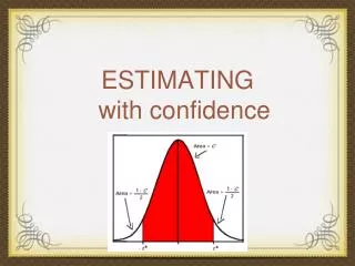
Confidence Interval • A level C confidence interval for a parameter has two parts. • An interval calculated from the data, usually in the form (estimate plus or minus margin of error) • A confidence level C, which gives the long term proportion that the interval will capture the true parameter value in repeated samples.
Conditions for Confidence Intervals • the data come from an SRS or well designed experiment from the population of interest • the sample distribution is approximately normal
Four Step Process (Inference Toolbox) • Step 1 (Pop and para) • Define the population and parameter you are investigating • Step 2 (Conditions) • Do we biased data? • If SRS, we’re good. Otherwise PWC. • Do we independent sampling? • If pop>10n, we’re good. Otherwise PWC. • Do we have a normal distribution? • If pop is normal or n>25, we’re good. Otherwise, PWC.
Four Step Process (Inference Toolbox) • Step 3 (Calculations) • Find z* based on your confidence level. If you are not given a confidence level, use 95% • Calculate CI. • Step 4 (Interpretation) • “With ___% confidence, we believe that the true mean is between (lower, upper)”
Confidence interval behavior • To make the margin of error smaller… • make z* smaller, which means you have lower confidence • make n bigger, which will cost more
Confidence interval behavior • If you know a particular confidence level and ME, you can solve for your sample size.
Company management wants a report screen tensions which have standard deviation of 43 mV. They would like to know how big the sample has to be to be within 5 mV with 95% confidence? You need a sample size of at least 285. Example
Mantras • “Interpret 80% confidence interval of (454,467)” • With 80% confidence we believe that the true mean of California senior SAT-M scores is between 454 and 467. • “Interpret 80% confidence” • If we use these methods repeatly, 80% of the time our confidence interval captures the true mean. • Probability
Assignment • Exercises 10.1 to 10.25 every other odd