Download

1 / 93
930 likes | 1.3k Views
Machine Learning” Notes 2. Dr. Alper Özpınar. Training , Validating and Testing Data.

E N D
Machine Learning”Notes 2 Dr. Alper Özpınar
Training, Validating andTesting Data • To make a model, we first need data that has an underlying relationship. For this example, we will create our own simple dataset with x-values (features) and y-values (labels). An important part of our data generation is adding random noise to the labels. In any real-world process, whether natural or man-made, the data does not exactly fit to a trend. There is always noise or other variables in the relationship we cannot measure.
Overfitting in Machine Learning • Overfitting refers to a model that models the training data too well. • Overfitting happens when a model learns the detail and noise in the training data to the extent that it negatively impacts the performance of the model on new data. This means that the noise or random fluctuations in the training data is picked up and learned as concepts by the model. The problem is that these concepts do not apply to new data and negatively impact the models ability to generalize. • Overfitting is more likely with nonparametric and nonlinear models that have more flexibility when learning a target function. As such, many nonparametric machine learning algorithms also include parameters or techniques to limit and constrain how much detail the model learns. • For example, decision trees are a nonparametric machine learning algorithm that is very flexible and is subject to overfitting training data. This problem can be addressed by pruning a tree after it has learned in order to remove some of the detail it has picked up.
Underfitting in Machine Learning • Underfitting refers to a model that can neither model the training data nor generalize to new data. • An underfit machine learning model is not a suitable model and will be obvious as it will have poor performance on the training data. • Underfitting is often not discussed as it is easy to detect given a good performance metric. The remedy is to move on and try alternate machine learning algorithms. Nevertheless, it does provide a good contrast to the problem of overfitting.
Classification Using Distance • Place items in class to which they are “closest”. • Must determine distance between an item and a class. • Classes represented by • Centroid: Central value. • Medoid: Representative point. • Individual points • Algorithm: KNN
K Nearest Neighbor (KNN): • Training set includes classes. • Examine K items near item to be classified. • New item placed in class with the most number of close items. • O(q) for each tuple to be classified. (Here q is the size of the training set.)
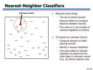
Compute Distance Test Record Training Records Choose k of the “nearest” records Nearest Neighbor Classifiers • Basic idea: • If it walks like a duck, quacks like a duck, then it’s probably a duck Data Mining: Concepts and Techniques
new Nearest neighbor method • Majority vote within the k nearest neighbors K= 1: brown K= 3: green Data Mining: Concepts and Techniques
Nearest-Neighbor Classifiers • Requires three things • The set of stored records • Distance Metric to compute distance between records • The value of k, the number of nearest neighbors to retrieve • To classify an unknown record: • Compute distance to other training records • Identify k nearest neighbors • Use class labels of nearest neighbors to determine the class label of unknown record (e.g., by taking majority vote) Data Mining: Concepts and Techniques
Definition of Nearest Neighbor K-nearest neighbors of a record x are data points that have the k smallest distance to x Data Mining: Concepts and Techniques
1 nearest-neighbor Voronoi Diagram Data Mining: Concepts and Techniques
Nearest Neighbor Classification • Compute distance between two points: • Euclidean distance • Determine the class from nearest neighbor list • take the majority vote of class labels among the k-nearest neighbors • Weigh the vote according to distance • weight factor, w = 1/d2 Data Mining: Concepts and Techniques
Nearest Neighbor Classification… • Choosing the value of k: • If k is too small, sensitive to noise points • If k is too large, neighborhood may include points from other classes Data Mining: Concepts and Techniques
Nearest Neighbor Classification… • Scaling issues • Attributes may have to be scaled to prevent distance measures from being dominated by one of the attributes • Example: • height of a person may vary from 1.5m to 1.8m • weight of a person may vary from 90lb to 300lb • income of a person may vary from $10K to $1M Data Mining: Concepts and Techniques
Nearest Neighbor Classification… • Problem with Euclidean measure: • High dimensional data • curse of dimensionality • Can produce counter-intuitive results 1 1 1 1 1 1 1 1 1 1 1 0 1 0 0 0 0 0 0 0 0 0 0 0 vs 0 1 1 1 1 1 1 1 1 1 1 1 0 0 0 0 0 0 0 0 0 0 0 1 d = 1.4142 d = 1.4142 • Solution: Normalize the vectors to unit length Data Mining: Concepts and Techniques
Nearest neighbor Classification… • k-NN classifiers are lazy learners • It does not build models explicitly • Unlike eager learners such as decision tree induction and rule-based systems • Classifying unknown records are relatively expensive Data Mining: Concepts and Techniques
Discussion on the k-NN Algorithm • The k-NN algorithm for continuous-valued target functions • Calculate the mean values of the k nearest neighbors • Distance-weighted nearest neighbor algorithm • Weight the contribution of each of the k neighbors according to their distance to the query point xq • giving greater weight to closer neighbors • Similarly, for real-valued target functions • Robust to noisy data by averaging k-nearest neighbors • Curse of dimensionality: distance between neighbors could be dominated by irrelevant attributes. • To overcome it, axes stretch or elimination of the least relevant attributes. Data Mining: Concepts and Techniques
categorical categorical continuous class Decision Trees Splitting Attributes Refund Yes No NO MarSt Married Single, Divorced TaxInc NO < 80K > 80K YES NO Model: Decision Tree Training Data
NO Another Example of Decision Tree categorical categorical continuous class Single, Divorced MarSt Married NO Refund No Yes TaxInc < 80K > 80K YES NO There could be more than one tree that fits the same data!
Decision Tree Classification Task Decision Tree
Refund Yes No NO MarSt Married Single, Divorced TaxInc NO < 80K > 80K YES NO Apply Model to Test Data Test Data Start from the root of tree.
Refund Yes No NO MarSt Married Single, Divorced TaxInc NO < 80K > 80K YES NO Apply Model to Test Data Test Data
Apply Model to Test Data Test Data Refund Yes No NO MarSt Married Single, Divorced TaxInc NO < 80K > 80K YES NO
Apply Model to Test Data Test Data Refund Yes No NO MarSt Married Single, Divorced TaxInc NO < 80K > 80K YES NO
Apply Model to Test Data Test Data Refund Yes No NO MarSt Married Single, Divorced TaxInc NO < 80K > 80K YES NO
Apply Model to Test Data Test Data Refund Yes No NO MarSt Assign Cheat to “No” Married Single, Divorced TaxInc NO < 80K > 80K YES NO
Decision Tree Classification Task Decision Tree
Decision Tree Induction • Many Algorithms: • Hunt’s Algorithm (one of the earliest) • CART • ID3, C4.5 • SLIQ,SPRINT
General Structure of Hunt’s Algorithm • Let Dt be the set of training records that reach a node t • General Procedure: • If Dt contains records that belong the same class yt, then t is a leaf node labeled as yt • If Dt is an empty set, then t is a leaf node labeled by the default class, yd • If Dt contains records that belong to more than one class, use an attribute test to split the data into smaller subsets. Recursively apply the procedure to each subset. Dt ?
Refund Refund Yes No Yes No Don’t Cheat Marital Status Don’t Cheat Marital Status Single, Divorced Refund Married Married Single, Divorced Yes No Don’t Cheat Taxable Income Cheat Don’t Cheat Don’t Cheat Don’t Cheat < 80K >= 80K Don’t Cheat Cheat Hunt’s Algorithm Don’t Cheat
Tree Induction • Greedy strategy. • Split the records based on an attribute test that optimizes certain criterion. • Issues • Determine how to split the records • How to specify the attribute test condition? • How to determine the best split? • Determine when to stop splitting
Tree Induction • Greedy strategy. • Split the records based on an attribute test that optimizes certain criterion. • Issues • Determine how to split the records • How to specify the attribute test condition? • How to determine the best split? • Determine when to stop splitting
How to Specify Test Condition? • Depends on attribute types • Nominal • Ordinal • Continuous • Depends on number of ways to split • 2-way split • Multi-way split
CarType Family Luxury Sports CarType CarType {Sports, Luxury} {Family, Luxury} {Family} {Sports} Splitting Based on Nominal Attributes • Multi-way split: Use as many partitions as distinct values. • Binary split: Divides values into two subsets. Need to find optimal partitioning. OR
Size Small Large Medium Size Size Size {Small, Medium} {Small, Large} {Medium, Large} {Medium} {Large} {Small} Splitting Based on Ordinal Attributes • Multi-way split: Use as many partitions as distinct values. • Binary split: Divides values into two subsets. Need to find optimal partitioning. • What about this split? OR
Splitting Based on Continuous Attributes • Different ways of handling • Discretization to form an ordinal categorical attribute • Static – discretize once at the beginning • Dynamic – ranges can be found by equal interval bucketing, equal frequency bucketing (percentiles), or clustering. • Binary Decision: (A < v) or (A v) • consider all possible splits and finds the best cut • can be more compute intensive
Tree Induction • Greedy strategy. • Split the records based on an attribute test that optimizes certain criterion. • Issues • Determine how to split the records • How to specify the attribute test condition? • How to determine the best split? • Determine when to stop splitting
How to determine the Best Split Before Splitting: 10 records of class 0, 10 records of class 1 Which test condition is the best?
How to determine the Best Split • Greedy approach: • Nodes with homogeneous class distribution are preferred • Need a measure of node impurity: Non-homogeneous, High degree of impurity Homogeneous, Low degree of impurity
Measures of Node Impurity • Gini Index • Entropy • Misclassification error
M0 M2 M3 M4 M1 M12 M34 How to Find the Best Split Before Splitting: A? B? Yes No Yes No Node N1 Node N2 Node N3 Node N4 Gain = M0 – M12 vs M0 – M34
Measure of Impurity: GINI • Gini Index for a given node t : (NOTE: p( j | t) is the relative frequency of class j at node t). • Maximum (1 - 1/nc) when records are equally distributed among all classes, implying least interesting information • Minimum (0.0) when all records belong to one class, implying most interesting information
Examples for computing GINI P(C1) = 0/6 = 0 P(C2) = 6/6 = 1 Gini = 1 – P(C1)2 – P(C2)2 = 1 – 0 – 1 = 0 P(C1) = 1/6 P(C2) = 5/6 Gini = 1 – (1/6)2 – (5/6)2 = 0.278 P(C1) = 2/6 P(C2) = 4/6 Gini = 1 – (2/6)2 – (4/6)2 = 0.444