Download
1 / 42
420 likes | 582 Views
Introduction to Turing Machines. Juan Carlos Guzmán CS 6413 Theory of Computation Southern Polytechnic State University. What Are Programs?. Programs can be thought of as implementation of languages (or properties) P ( x ) = yes, if x L P P ( x ) = no, otherwise

E N D
Introduction to Turing Machines Juan Carlos Guzmán CS 6413 Theory of Computation Southern Polytechnic State University
What Are Programs? • Programs can be thought of as implementation of languages (or properties) • P(x) = yes, if xLP • P(x) = no, otherwise • How do we describe programs • Programs are themselves finite strings
On Counting Languages • Consider Σ = {0,1} • Σ* = {ε,0,1,00,01,10,11,000,…} • If L is a language over Σ • then L Σ* • If LΣ is the set of all languages over Σ • LΣ= P (Σ*) (or 2Σ*) (parts of Σ*)
On Counting Languages • It is a well-known mathematical fact that, for any set A |A| < |2A| • In our case |Σ*| < | LΣ| • However • Programs are strings • They solve problems on strings (languages)
On Counting Languages • There must be languages that cannot be described • In fact, for any language described, there are infinitely many that are not described
Decidable Problem • A problem is decidable if there is an algorithm that correctly answers “yes” or “no” to each instance of the problem • Otherwise, the problem is undecidable
The Halting Problem • Determining whether a program terminates for a given input is undecidable
The Halting Problem • Let’s assume there is such a program, called halting • halting: Program × Input {yes,no} • There is another program looping, that does not terminate • looping: Input _|_
The Halting Problem • H1 = P . halting(P,P) • H2 = P . if halting(P,P) then looping(P) else “yes” What is the answer of H2(H2)
Paradox • If H2 really halts on H2, then it will loop • If H2 loops, then it really should halt • The paradox arises from assuming the existence of the halting program
Problem Reduction • Suppose P1 is undecidable • We want to prove that P2 is also undecidable • We need to find a transformation that would take any instance of P1 into an instance of P2 • We have thus proven that P2 is undecidable
Church-Turing Thesis • All general-purpose models of computation have the same power • they compute exactly the same functions • partial recursive functions
Turing Machine • Finite set of states • Unbounded tape • blank characters, except • a finite string (input) in the tape • Tape head • always scanning one cell • initially scanning leftmost character of input • Movement • moves left or right • reads the current character on the tape • writes a character symbol
Turing Machine • M = (Q,Σ,Γ,δ,q0,B,F ), where • Q is the set of states • Σ is the set of input symbols • Γ is the set of tape symbols (Σ Γ) • δ is the transition function • δ: (Q × Γ) (Q × Γ × {left,right}) • q0 is the starting state • B is the blank symbol (B Γ - Σ) • F is the set of final states
… B X1 X2 … Xi … Xn B … q Instantaneous Description • An instantaneous description is a sequence X1X2…Xi-1qXi…Xn, where • Xk in Γ • q in Q • All Xi’s are nonblank, except when q is at one of the extremes, when there may be a sequence of blanks between q and the string • The elements not represented in the tape are all blank • In this description, q is scanning Xi, so, if we were more sophisticated, we could write
Movement Relation (├) • If the current ID of the machine is X1X2…Xi-1qXi…Xn • If δ(q,Xi) = (p,Y,left) • X1X2…Xi-1qXi…Xn├ X1X2…Xi-2pXi-1Y…Xn • If δ(q,Xi) = (p,Y,right) • X1X2…Xi-1qXi…Xn├ X1X2…Xi-1YpXi+1…Xn • We will not notate blanks to the end of the ID, so
Example (0n1n) Y/Y 0/0 Y/Y 0/0 start 0/X B/B Y/Y 1/Y q4 q3 q0 q1 q2 X/X Y/Y
Language of a Turing Machine • Acceptance by final state • q0w ├p with p F • Acceptance by halting
Programming Techniques • Storage in the State • Multiple tracks • Subroutines
Storage in the State • Store information along with the state • Otherwise, the TM really can only store info in the tape q,A,B,C … B X1 X2 … Xi … Xn B … q A C D
… B X1 X2 … Xi … Xl B … … B Y1 Y2 … Yj … Ym B … … B Z1 Z2 … Zk … Zn B … q Multiple Tracks • Each “symbol” is actually a tuple of several symbols • Initially, only the upper track contains information
Subroutines • TM’s do not have any abstraction mechanism – no call/return pair • We can reason about code with some level of abstraction (e.g. swap), and splice the operation every time it is used
Extensions to Turing Machines • Multi-tape Turing Machine • Nondeterministic Turing Machine
Multi-Tape Turing Machines • Several tapes • Ability to move each of them independently • The initial string is in the first tape • All other tapes are initially empty • There is one head per tape – each tape • Scans an input symbol • Upon transition • Writes a new symbol • moves left, right, or remains stationary
… B X1 X2 … Xi … Xl B … … B Y1 Y2 … Yj … Ym B … Multi-Tape Turing Machines … B Z1 Z2 … Zk … Zn B … q
Multi-Tape Turing Machines • Are many tapes better than one? • Does a ‘multi-tape TM’ have more power than a (single tape) TM? • Can it compute more functions? • See Turing-Church Thesis • A ‘multi-tape TM’ computes exactly the same functions as a (single tape) TM
Multi-Tape Turing Machines • A (single tape) TM is already a multi-tape TM, with only one tape • A k-tape TM can be simulated by a (single tape) Turing Machine • with 2k tracks • k tracks to store the k tapes • k corresponding tracks to mark the positions of the heads of the multi-tape TM • a stored value meaning “the number of heads are to the left of the current position”
Nondeterministic Turing Machines • Delta(q,X) can be a set of triplets, rather than a single triplet • Therefore, the machine may have a choice of movements on certain configurations
Nondeterministic Turing Machines • Nondeterminstic Turing Machines (NTM) accept the same class of languages as the deterministic Turing Machines (DTM) • Use a two-tape deterministic TM to simulate a NTM • Use one tape to keep a queue of ID’s • Use the other as scratch to simulate executions of the NTM • Separate the ID’s and mark current one • Each NTM is emulated by a different DTM x ID1 * ID2 * ID3 * ID4 … … q
Nondeterministic Turing Machines • To execute current ID – find q and a • Encoded in the machine is knowledge on how many different movements it can do on such input • For each choice • Copy the ID into the scratch tape • Do the corresponding movement • Copy the resulting ID to the end of the first tape • Advance current ID marker x ID1 * ID2 * ID3 * ID4 * ID5 * ID6* ID7 … … q
Running Time of Simulated Machines • Machines run in simulation take more steps to accept a string than if they were running natively • Multi-tape by One-tape TM • O(n2) • Nondeterministic to Deterministic TM • exponential
Restricted Turing Machines • Turing Machines with semi-infinite tapes • Multi-stack machines • Counter machines
Turing Machines with Semi-Infinite Tapes • There is the concept of the “beginning of the tape” • Simulate the two-way infiniteness by having a two-track tape X0 X1 X2 … Xi … * X-1 X-2 … X-i … q
Multi-Stack Machines • These are PDA’s with multiple stacks • Each stack is handled independently • An symbol is popped • A group of symbols is pushed • Two-stack machines recognize the same class of languages as Turing Machines
Counter Machines • Similar to stack machines, but more restricted • Instead of stacks, the machines have counters, that can hold any positive value, or zero, and can be incremented or decremented independently
Turing Machines and Computers • A computer can simulate a Turing Machine (although with some difficulty) • A Turing Machine can simulate a computer (in polynomial time)
Computer Simulation of a Turing Machine • No computer with a finite amount of memory is able to simulate a Turing Machine • Consider that the hard drive is the tape – you can buy very large ones, but they are finite • A TM can solve problems that require more memory than the memory available to the computer • Consider a string so awfully large that is larger than the computer’s memory
Computer Simulation of a Turing Machine • Assume • Unbounded amounts of removable media • Each disk represents a segment of the tape • The computer can have one segment at any given time Computer Tape to the left Tape to the right
Turing Machine Simulation of a Computer • A computer can be simulated by a multi-tape Turing Machine Memory Instruction Counter Memory Address Input File Scratch … q
Turing Machine Simulation of a Computer • The good news … • The simulation only takes polynomial time!
Some languages cannot be not recognized Some languages are recognized, but not reasonably fast Polynomial time, vs. Exponential time Languages Recognized by Machines All languages TM NPDA DPDA FA