Download
1 / 53
550 likes | 628 Views
Turing Machines. Everything is an Integer Countable and Uncountable Sets Turing Machine Definition. Integers, Strings, and Other Things. Data types have become very important as a programming tool. But at another level, there is only one type, which you may think of as integers or strings.

E N D
Turing Machines Everything is an Integer Countable and Uncountable Sets Turing Machine Definition
Integers, Strings, and Other Things • Data types have become very important as a programming tool. • But at another level, there is only one type, which you may think of as integers or strings. • Key point: Strings that are programs are just another way to think about the same one data type.
Example: Text • Strings of ASCII or Unicode characters can be thought of as binary strings, with 8 or 16 bits/character. • Binary strings can be thought of as integers. • It makes sense to talk about “the i-th string.”
Binary Strings to Integers • There’s a small glitch: • If you think simply of binary integers, then strings like 101, 0101, 00101,… all appear to be “the fifth string.” • Fix by prepending a “1” to the string before converting to an integer. • Thus, 101, 0101, and 00101 are the 13th, 21st, and 37th strings, respectively.
Example: Images • Represent an image in (say) GIF. • The GIF file is an ASCII string. • Convert string to binary. • Convert binary string to integer. • Now we have a notion of “the i-th image.”
Example: Proofs • A formal proof is a sequence of logical expressions, each of which follows from the ones before it. • Encode mathematical expressions of any kind in Unicode. • Convert expression to a binary string and then an integer.
Proofs – (2) • But a proof is a sequence of expressions, so we need a way to separate them. • Also, we need to indicate which expressions are given.
Proofs – (3) • Quick-and-dirty way to introduce new symbols into binary strings: • Given a binary string, precede each bit by 0. • Example: 101 becomes 010001. • Use strings of two or more 1’s as the special symbols. • Example: 111 = “the following expression is given”; 11 = “end of expression.”
A given expression follows End of expression Expression End A given expression follows An ex- pression Notice this 1 could not be part of the “end” Example: Encoding Proofs 1110100011111100000101110101…
Example: Programs • Programs are just another kind of data. • Represent a program in ASCII. • Convert to a binary string, then to an integer. • Thus, it makes sense to talk about “the i-th program.” • Hmm…There aren’t all that many programs.
Finite Sets • Intuitively, a finite set is a set for which there is a particular integer that is the count of the number of members. • Example: {a, b, c} is a finite set; its cardinality is 3. • It is impossible to find a 1-1 mapping between a finite set and a proper subset of itself.
Infinite Sets • Formally, an infinite set is a set for which there is a 1-1 correspondence between itself and a proper subset of itself. • Example: the positive integers {1, 2, 3,…} is an infinite set. • There is a 1-1 correspondence 1<->2, 2<->4, 3<->6,… between this set and a proper subset (the set of even integers).
Countable Sets • A countable set is a set with a 1-1 correspondence with the positive integers. • Hence, all countable sets are infinite. • Example: All integers. • 0<->1; -i <-> 2i; +i <-> 2i+1. • Thus, order is 0, -1, 1, -2, 2, -3, 3,… • Examples: set of binary strings, set of Java programs.
Example: Pairs of Integers • Order the pairs of positive integers first by sum, then by first component: • [1,1], [2,1], [1,2], [3,1], [2,2], [1,3], [4,1], [3,2],…, [1,4], [5,1],… • Interesting fact: this same proof means that rational numbers are countable.
Enumerations • An enumeration of a set is a 1-1 correspondence between the set and the positive integers. • Thus, we have seen enumerations for strings, programs, proofs, and pairs of integers.
How Many Languages? • Are the languages over {0,1}* countable? • No; here’s a proof. • Suppose we could enumerate all languages over {0,1}* and talk about “the i-th language.” • Consider the language L = { w | w is the i-th binary string and w is not in the i-th language}.
Lj x j-th Proof – Continued • Clearly, L is a language over {0,1}*. • Thus, it is the j-th language for some particular j. • Let x be the j-th string. • Is x in L? • If so, x is not in L by definition of L. • If not, then x is in L by definition of L. Recall: L = { w | w is the i-th binary string and w is not in the i-th language}.
Diagonalization Picture Strings 1 2 3 4 5 … … 1 0 1 1 0 1 2 1 Languages 3 0 4 0 1 5 … …
Can’t be a row – it disagrees in an entry of each row. Diagonalization Picture Strings Flip each diagonal entry 1 2 3 4 5 … … 0 0 1 1 0 1 2 0 Languages 3 1 4 1 0 5 … …
Proof – Concluded • We have a contradiction: x is neither in L nor not in L, so our sole assumption (that there was an enumeration of the languages) is wrong. • Thus, there are (way) more languages than programs. • E.g., there are languages with no membership algorithm.
Non-constructive Arguments • We have shown the existence of a language with no algorithm to test for membership, but we have not exhibited a particular language with that property. • A proof that shows only that something exists without showing a way to find it or giving a specific example is a non-constructive argument.
Turing-Machine Theory • The purpose of the theory of Turing machines was to prove that certain specific languages have no algorithm.
Picture of a Turing Machine Action: based on the state and the tape symbol under the head: change state, rewrite the symbol and move the head one square. State . . . . . . A B C A D Infinite tape with squares containing tape symbols chosen from a finite alphabet
Why Turing Machines? • Why not deal with C programs or something like that? • Answer: You can, but it is easier to prove things about TM’s, because they are so simple. • And yet they are as powerful as any computer. • More so, in fact, since they have infinite memory.
Turing-Machine Definition • A TM is described by: • A finite set of states (Q, typically). • An input alphabet (Σ, typically). • A tape alphabet (Γ, typically; contains Σ), which includes a blank symbol, B, not in Σ. • Entire tape except for the input is initially blank. • A transition function (δ, typically). • A start state (q0, in Q, typically). • An final (accept) state (f or qaccept, typically). • A reject state (r or qreject, typically).
The Transition Function • Takes two arguments: • A state, in Q. • A tape symbol in Γ. • δ(q, Z) is either undefined or a triple of the form (p, Y, D). • p is a state. • Y is the new tape symbol. • D is a direction, L or R.
Actions of the TM • If δ(q, Z) = (p, Y, D) then, in state q, scanning Z under its tape head, the TM: • Changes the state to p. • Replaces Z by Y on the tape. • Moves the head one square in direction D. • D = L: move left; D = R; move right.
Conventions • a, b, … are input symbols. • …, X, Y, Z are tape symbols. • …, w, x, y, z are strings of input symbols. • , ,… are strings of tape symbols.
Language of a Turing Machine • Once a TM has entered either the accept state or reject state, it halts. • Initially, the input for a TM, M, is on its tape, its head is pointing to the first character of the input (or B if it is null), and M is in its start state • An input string, w, is in the language of M if the actions of M with w as its input results in it halting in the accept state.
Example: Turing Machine • This TM scans its input right, turning each 0 into a 1. • If it ever finds a 1, it goes to final reject state r, goes right on square, and halts. • If it reaches a blank, it changes moves left and accepts. • Its language is 0*
Example: Turing Machine – (2) • States = {q (start), f (accept), r (reject)}. • Input symbols = {0, 1}. • Tape symbols = {0, 1, B}. • δ(q, 0) = (q, 1, R). • δ(q, 1) = (r, 1, R). • δ(q, B) = (f, B, L).
q Simulation of TM δ(q, 0) = (q, 1, R) δ(q, 1) = (r, 1, R) δ(q, B) = (f, B, L) . . . B B 0 0 B B . . .
q Simulation of TM δ(q, 0) = (q, 1, R) δ(q, 1) = (r, 1, R) δ(q, B) = (f, B, L) . . . B B 1 0 B B . . .
q Simulation of TM δ(q, 0) = (q, 1, R) δ(q, 1) = (r, 1, R) δ(q, B) = (f, B, L) . . . B B 1 1 B B . . .
f Simulation of TM δ(q, 0) = (q, 1, R) δ(q, 1) = (r, 1, R) δ(q, B) = (f, B, L) The TM halts and accepts. (So “00” is in its language.) . . . B B 1 1 B B . . .
q Simulation of TM – on 001 δ(q, 0) = (q, 1, R) δ(q, 1) = (r, 1, R) δ(q, B) = (f, B, L) . . . B B 0 0 1 B . . .
q Simulation of TM – on 001 δ(q, 0) = (q, 1, R) δ(q, 1) = (r, 1, R) δ(q, B) = (f, B, L) . . . B B 1 0 1 B . . .
q Simulation of TM – on 001 δ(q, 0) = (q, 1, R) δ(q, 1) = (r, 1, R) δ(q, B) = (f, B, L) . . . B B 1 1 1 B . . .
r Simulation of TM δ(q, 0) = (q, 1, R) δ(q, 1) = (r, 1, R) δ(q, B) = (f, B, L) The TM halts and rejects. (So “001” is not in its language.) . . . B B 1 1 1 B . . .
Turing Machine’s Can Have Infinite Loops • Once a TM has entered either the accept state or reject state, it halts. • But there is no rule that a TM must halt. • Turing Machines can have infinite loops.
A ”Loopy” Turing Machine • States = {q (start), f (accept), r (reject)}. • Input symbols = {0, 1}. • Tape symbols = {0, 1, B}. • δ(q, 0) = (q, 0, R). • δ(q, 1) = (q, 1, L). • δ(q, B) = (f, B, L).
q Simulation of Loopy TM δ(q, 0) = (q, 0, R) δ(q, 1) = (q, 1, L) δ(q, B) = (f, B, L) . . . B B 0 1 B B . . .
q Simulation of Loopy TM δ(q, 0) = (q, 0, R) δ(q, 1) = (q, 1, L) δ(q, B) = (f, B, L) . . . B B 0 1 B B . . .
q Simulation of Loopy TM δ(q, 0) = (q, 0, R) δ(q, 1) = (q, 1, L) δ(q, B) = (f, B, L) . . . B B 0 1 B B . . .
q Simulation of Loopy TM δ(q, 0) = (q, 0, R) δ(q, 1) = (q, 1, L) δ(q, B) = (f, B, L) The TM never halts in this case. But notice that it still accepts the language 0* . . . B B 0 1 B B . . .
Instantaneous Descriptions of a Turing Machine • Initially, a TM has a tape consisting of a string of input symbols surrounded by an infinity of blanks in both directions. • The TM is in the start state, and the head is at the leftmost input symbol.
TM ID’s – (2) • An ID is a string q, where is the tape between the leftmost and rightmost nonblanks (inclusive). • The state q is immediately to the left of the tape symbol scanned. • If q is at the right end, it is scanning B. • If q is scanning a B at the left end, then consecutive B’s at and to the right of q are part of .
TM ID’s – (3) • As for PDA’s we may use symbols ⊦ and ⊦* to represent “becomes in one move” and “becomes in zero or more moves,” respectively, on ID’s. • Example: The moves of the previous TM are q00⊦0q0⊦00q⊦0q01⊦00q1⊦000f
Formal Definition of Moves • If δ(q, Z) = (p, Y, R), then • qZ⊦Yp • If Z is the blank B, then also q⊦Yp • If δ(q, Z) = (p, Y, L), then • For any X, XqZ⊦pXY • In addition, qZ⊦pBY
Formal Definition of the Language of a TM • Recall that once a TM has entered either the accept state or reject state, it halts. • If M is a Turing Machine, the language accepted by M is: L(M) = {w | q0w⊦*I, where I is an ID with the accept state}.