Download

1 / 20
200 likes | 212 Views
Online Monitoring of Software System Reliability. Stefano Russo The Mobilab Research Group Computer Science and Systems department University of Naples Federico II 80125 Naples, Italy Stefano.Russo@unina.it. Kishor S. Trivedi Dept. of Electrical & Computer Engineering Duke University

E N D
Online Monitoring of Software System Reliability Stefano Russo The Mobilab Research Group Computer Science and Systems department University of Naples Federico II 80125 Naples, Italy Stefano.Russo@unina.it Kishor S. Trivedi Dept. of Electrical & Computer Engineering Duke University Durham, NC 27708 USA kst@ee.duke.edu Roberto Pietrantuono The Mobilab Research Group Computer Science and Systems department University of Naples Federico II 80125 Naples, Italy roberto.pietrantuono@unina.it
Context Software Reliability Assuring software reliability is gaining importance “Reactive” vs. “proactive” policies for reliability/availability assurance “Proactive” means acting before the system failure occurrence by attempting to forecast the failure and by taking proper actions to avoid the system failure Software Reliability Evaluation Proactively acting to assure a reliability level at runtime requires evaluating reliability during the execution OUR GOAL: propose a solution for Online Software Reliability Evaluation
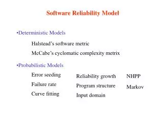
Model-based Compositional approaches Decomposition/aggregation Derived from high level specification A relevant class is Architecture-based models State-based Path-based Additive Reliability usually estimated statically in the development phase Models can be not enough representative of actual runtime behavior => i.e., inaccuracy due to the necessary assumptions Reliability Evaluation Solutions
Reliability Evaluation Solutions Measurements-based • Relies on operational data and statistical inference techniques • However, real data are not always available • Few insights about the internal dependencies among system components • They are not suited for predictions on reliability aimed at taking proactive actions
Proposed Approach A method to estimate reliability at runtime, in two phases: A preliminary modeling phase, based on the development phase An architecture-based modelis used to give an estimate at software release A refinement phase, where data that become available as the execution proceeds are used to refine the model results A dynamic analysis tool is used to continuously evaluate the “impact” of operational data on the current estimate Real operational data are used to counterbalance potential errors due to the model simplifications and assumptions Key idea: combine modeling power with operational data representativeness
Modelling Phase • Represent the system as an absorbing DTMC where • states are software components • transitions are the flow of control among them • With this model, reliability can be estimated as: E[Rsys] ~ (Πin-1RiE[X1,i]) * Rn • E[X1,i]is the expected number of visits from component 1 to i, a.k.a. Visit Counts • Riare component reliabilities Ri estimated as 1- limni fi /ni with fibeing the number of failures and ni the number of executions in N randomly generated test cases
Modelling Phase (2) • What affects the inaccuracy of this estimation are the assumptions on which it is based, e.g.: • First-order Markov chain • Operational profile mismatch • Components fail independently To overcome these limitations a runtime refinement phase is carried out • Errors on visit counts values • Errors on individual component reliability
Runtime Phase • As for the error type I, we record real “visits” among components and give an estimate of the random variables Vi • As for the error type II, we use dynamic analysis tool (Daikon) to: Testing Phase Runtime Phase • Detect at runtime deviations from the defined expected behavior. • Each time components interact with each other in unexpected ways, a “penalty function” properly lowers the Ri value • Instrument and Monitor components • describe their behavior by observing interactions and building invariants on exchanged value • (i.e., we build the “expected” behavioral model)
Reliability Degradation Estimate • Component reliabilities need to be reduced to consider new online behaviors, by a penalty function • However, a deviation (violation) can be either an incorrect behavior or afalse-positive • At each time T a “penalty value” has to be chosen • It considers a risk associated with the set of all violations occurred in that interval (called Risk Factor, RF) Risk that the observed set of violations are incorrect behaviors
Reliability Degradation Estimate • The risk that observed violations represent incorrect behaviors depends on: • The number of occurred violations • The number of distinct program points that experienced violations • The robustness of the model (i.e., the confidence that can be given to the invariants) RFi =#Violation / #MaxViolation * #DistinctPoints / #MonitoredPoints RnONLINEi = R(n-1)ONLINEi - R(n-1)ONLINEi * RFi * W • W is a parameter to tune how much RF has to impact on penalization: • Related to the confidence parameter in the built invariants
Evaluation Case-study: a queuing systems simulator Based on javasim • 5426 LoC (without the jFreeChart code) • Components Identification: we considered Java packages as component granularity, getting to a set of 12 components Based on jFreeChart
Results Evaluation Procedure Testing Phase 180 test cases generated randomly picking valid combination of input parameters • E.g., interarrival time distribution, service time distribution, queue length, number of jobs, simulation method (independent replication or batch means), interarrival and service time means • Execution traces produced by Daikon • Ri estimated as 1 – Nf/N, with N = 360 additional executions • In our case REXP = 0.9972 • Usually leads to overestimations, since the systems is tested for its intended use • Runtime phase is responsible for adjusting it
Results Evaluation Procedure Runtime Phase Defined equivalence classes from input parameters and generated 3 operational profiles • a set of 30 executions per profile => the monitor is evaluated over 90 executions Violations and Visits are observed at each T => RFi and Vi estimation => RONLINEi computation => RONLINE (fixing REXP overestimation) Parameters setting
Results Experiments that caused an alarm triggering • 28 out of 90 executions reported violations w.r.t. the built invariants • 13 alarms raised • 9 false positives • 4 detected failures • 1 false negative (no alarm triggering) Results per Operational Profile
Results Operational Profile 2 Operational Profile 1 • Experiment 83 is a false-negative • Reliability can increase at some time intervals • changes in the usage => different Visit counts Operational Profile 3
Overhead Testing phase • Invariants construction => Daikon overhead • Execution traces production and invariant inference • The Daikon overhead is • Linear in the number of “true“ invariants • Linear to the test suite size • Linear in the instrumented points (proportional to the program size) • In our case it took 2283’’ (i.e., about 38’). It is an “offline” cost Runtime Phase • Runtime-checker insturmentation (before the execution) • Experienced a 1.04 slowing down in the average • Time to compute reliability equation (negligible)
Overhead • However … overhead is tightly related to the number of invariants to check and to the actual value taken by variables => highly variable • The number of invariants to check is known in advance => it can be used for predicting purposes • Several solutions to reduce instrumentation and invariants construction cost(at the expense of accuracy) • Reducing the number of instrumented points • Reducing the number of executions • Reducing the number of variables • The evaluation time interval T is also important => further trade-off parameter between accuracy and overhead • Dependent on application requirements
Future work In the future we aim to: Provide the system with the ability to automatically learn violations that did not result in a failure Consider an adaptive threshold value the monitor should set the threshold based on past experience (i.e., number of observed false-positives) and to the user needs (the desired level of false-positives/false-negatives) A combination with online diagnosis mechanisms is envisaged Consider and evaluate alternative dynamic analysis tools Extend experiments to more case studies
Thank You !! Questions? Comments? Contact info: roberto.pietrantuono@unina.it http://www.mobilab.unina.it