Software Reliability Models

1. Software Reliability Models

2. Reliability Estimation • It is very much desirable to know in quantifiable terms that what is the Reliability of the Software that has been delivered. • Most of the Reliability models uses testing to predict reliability, reliability estimation is the main product metrics of interest at the end of the testing phase. • Reliability of software often depends considerably on the quality of testing. • Hence, by assessing reliability we can also judge the quality of testing. • Basic Concepts and Definitions: • Reliability of a product specifies the probability of failure-free operation of that product for a given time duration. • Unreliability comes due to faults and failures. • Reliability is a probabilistic measure that assumes that the occurrence of failure of software is a random phenomenon. • Here, by randomness all that is meant is that the failure cannot be predicted accurately. • Reliability modelling is more meaningful for larger systems.

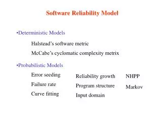
3. Musa’s Reliability Models Basic Concepts: Average Total Number of Failures: μ(τ), Failure Intensity – Number of Failures per time unit : λ(τ) Mean Time to Failure 1/λ(τ) • Two models • Basic • Logarithmic • Diff: Change in failure intensity per failure seen • Basic: decrement is constant • Logarithmic: decrement reduces 3

4. Reliability Model • Let us now discuss one particular reliability model Musa's basic execution time model. • This model focuses on failure intensity, failure intensity decreases with time, that is, as (execution) time increases, the failure intensity decreases. • Each failure causes the same amount of decrement in the failure intensity. That is, the failure intensity decreases with a constant rate with the number of failures. • Failure intensity (number of failures per unit time) as a function of the number of failures is given as: • Where is the initial failure intensity at the start of execution (i.e., at time t = 0), is the expected number of failures by the given time t, and is the total number of failures that would occur in infinite time.

5. Reliability Model • The total number of failures in infinite time is finite as it is assumed that on each failure, the fault in the software is removed. • As the total number of faults in a given software whose reliability is being modelled is finite, this implies that the number of failures is finite.

6. Reliability Model • The linear decrease in failure intensity as the number of failures observed increases is an assumption that is likely to hold for software for which the operational profile is uniform. • For software where the operational profile is such that any valid input is more or less equally likely, the assumption that the failure intensity decreases linearly generally holds. • The intuitive rationale is that if the operational profile is uniform, any failure can occur at any time and all failures will have the same impact in failure intensity reduction. • If the operational profile is not uniform, the failure intensity curves are ones whose slope decreases with the number of failures (i.e., each additional failure contributes less to the reduction in failure intensity). In such a situation the logarithmic model is better suited. • Note that the failure intensity decreases due to the nature of the software development process, in particular system testing, the activity in which reliability modelling is applied.

7. Reliability Model • Specifically, when a failure is detected during testing, the fault that caused the failure is identified and removed. It is removal of the fault that reduces the failure intensity. However, if the faults are not removed, as would be the situation if the software was already deployed in the field (when the failures are logged or reported but the faults are not removed), then the failure intensity would stay constant. • In this situation, the value of would stay the same as at the last failure that resulted in fault removal, and the reliability will be given by where T is the execution time. • The expected number of failures as a function of execution time T(i.e., expected number of failures by time T), in the model is assumed to have an exponential distribution. That is, • By substituting this value in the equation for A given earlier, we get the failure intensity as a function of time:

8. Reliability Model • A typical shape of the failure intensity as it varies with time is shown: • This reliability model has two parameters whose values are needed to predict the reliability of given software. These are the initial failure intensity and the total number of failures Unless the value of these are known, the model cannot be applied to predict the reliability of software. It would be very convenient if the values of these variables are applicable to all kind of software if varied can be easily calculated ,depending upon some software characteristic.

9. Reliability Model • However, no such simple method is currently available that is dependable. • The method that is currently used for all software reliability models is to estimate the value of these parameters for the particular software being modelled through the failure data for that software itself. In other words, the failure data of the software being modelled is used to obtain the value of these parameters. • The consequence of this fact is that, in general, for reliability modelling, the behaviour of the software system is carefully observed during system testing and data of failures observed during testing is collected up to some time T. • Then statistical methods are applied to this collected data to obtain the value of these parameters. Once the values of the parameters are known, the reliability (in terms of failure intensity) of the software can be predicted. These statistical methods require sufficient amount data, until that data is not available, values of the variables is not known.

10. Reliability Model • The Reason that we need reasonably large failure data , we cannot apply the reliability models to the small size software. • Also we cannot know the values the parameters precisely, we always have to estimate. This adds the uncertainty to the values and this further taken to the reliability estimates. • Let us assume that we start failure data collection with the testing that is T=0, This time should not start from where you are testing the modules, as these tests do not give the correct idea about the failure of the whole system. This is why data of unit testing or integration testing, where the whole system is not being tested, is not considered. • System testing, in which the entire system is being tested, is really the earliest point from where the data can be collected. • Some other values of interest can be used to decide whether enough testing has been done or some more testing is required to achieve the required reliability.

11. Reliability Model • Suppose the target reliability is specified in terms of desired failure intensity, Let the present failure intensity be Then the number of failures that we can expect to observe before the software achieves the desired reliability can be computed by computing which gives, • In other words, at any time we can now clearly say how many more failures we need to observe (and correct) before the software will achieve the target reliability. • Similarly, we can compute the additional time that needs to be spent before the target reliability is achieved. This is given by • we can expect that the software needs to be executed for more time before we will observe enough failures (and remove the faults corresponding to them) to reach the target reliability.

12. Basic (Linear) Model: • Assumption: decrement in failure intensity function derivative (w.r.t. number of expected failures) is constant • Consequence: failure intensity is function of average number of failures experienced at any given point in time failure probability Logarithmic Model: • Decrement per encountered failure decreases • Θ is a failure intensity decay parameter • Comparison of models: • Basic model assumes that there is a failure intensity - logarithmic model assumes convergence to 0 failure intensity • Basic model assumes a finite number of failures in the system - logarithmic model assumes infinite number 12

13. Reliability Models Logarithmic model Basic model l(m) = l0exp(-qm) l(m) = l0[1 - m/v0] q: failure intensity decay λ: Failure intensity λ0: Initial failure intensity at start of execution μ: Average total number of failures at a given point in time v0: Total number of failures over infinite time Initial failure intensity, l0 l: failure intensity Basic Log. v0 m: Mean failures exp.

14. Reliability Models Basic model Logarithmic model m(t) = (1/q).ln(l0qt + 1) m(t) = v0[1 – exp(-l0t/v0)] l(t) = l0/(l0qt + 1) l(t) = l0exp(-l0t/v0) l m Log. Log. v0 Basic Basic t t

15. Reliability Models Example: Assume that a program will experience 100 failures in infinite time. The initial failure intensity was 10 failures/CPU-hr, the present failure intensity is 3.68 failures/CPU-hour and our objective intensity is 0.000454 failure/CPU-hr. Predict the additional testing time to achieve the stated objective. Ans.: We know that l(t) = l0exp(-l0t/v0) At time t1, l(t1) = l0exp(-l0t1/v0) = lp At time t2, l(t2) = l0exp(-l0t2/v0) = lf t2 - t1 = (v0/ l0).ln(lp/ lf) v0 = 100 faults, l0 = 10 failures/CPU-hr lp = 3.68 failures/CPU-hr, lf = 0.000454 failure/CPU-hr Testing time = (t2 - t1 ) = 90 CPU-hr

16. Uses of Reliability • Uses of Model: • Measure reliability • Possible to measure for what modules increasing reliability will affect reliability of the system most • Can use a more effective testing strategy • Critical modules that have been shown to be reliable should be avoided changing • Not all bugs are equally costly 16