Download
1 / 60
600 likes | 736 Views
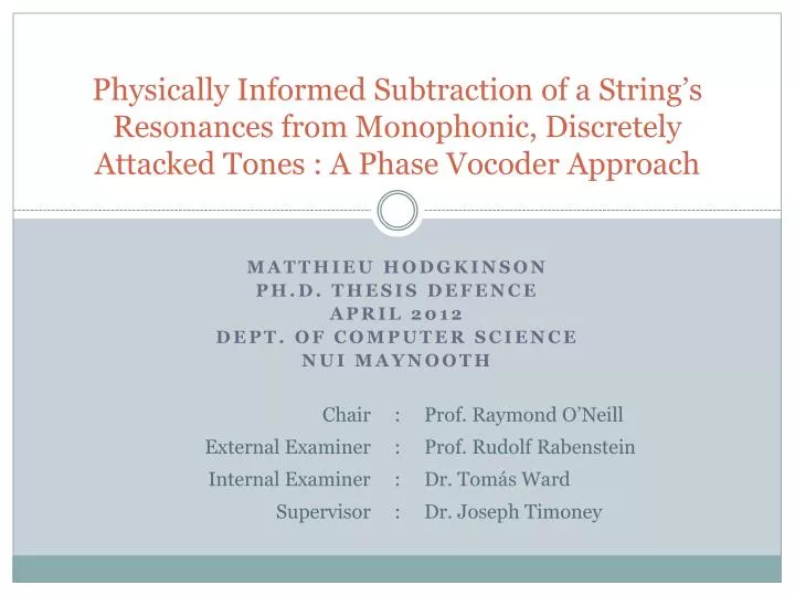
Physically Informed Subtraction of a String’s Resonances from Monophonic, Discretely Attacked Tones : A Phase Vocoder Approach. Matthieu Hodgkinson Ph.D. Thesis defence April 2012 Dept. Of computer science NUI Maynooth. String Extraction. Input (Viola Pizzicato). 1. Amplitude.

E N D
Physically Informed Subtraction of a String’s Resonances from Monophonic, Discretely Attacked Tones : A Phase Vocoder Approach MatthieuHodgkinson Ph.D. Thesis defence April 2012 Dept. Of computer science NUI Maynooth
String Extraction Input (Viola Pizzicato) 1 Amplitude Idea : subtract string resonances from monophonic, plucked or hit string tones. If input = string + excitation, then the remainder is input –string = excitation. Then “string extraction” reduces to “excitation extraction”. 0 -1 0 0.4958 Excitation 1 Amplitude 0 -1 0 0.4904 String 1 Amplitude 0 -1 0 0.4898
If input = string + excitation + other, then input – string = excitation + other. Now a few examples of other...
Environmental noise I Stratocaster Electric guitars : very short excitation (non-resonant body), electric buzz audible after string extraction. 0 Amplitude -1 0 2.7185 Time
Environmental noise II Martin (custom recording) 1 Accidental background noises in recording room. Amplitude 0 -1 0 1.9927 Time
Other strings Acoustic guitar (Open D) 1 Input Output Sometimes awkward to mute open strings. Non-muted strings respond to excitation and to vibrations of target string. Amplitude 0 0 1.5147 Time
Granulation and Extraction The string extraction uses a transparent Phase Vocoder scheme. The waveform is processed repeatedly over short time intervals. Each short-time output is added to the long-term output. This process is known as overlap-add. It is illustrated in the next few slides.
Granulation and Extraction Input 1 0.5 Waveform is multiplied by window to make grain. Sinusoidal components of string are subtracted. Residual is added to output. Process is repeated at regular time intervals, and residuals are added. 0 -0.5 -1 0 0.005 0.01 0.015 0.02 0.025 Output 1 window grain processed grain 0.5 0 -0.5 -1 0 0.005 0.01 0.015 0.02 0.025 Time (s)
Granulation and Extraction Input 1 0.5 Waveform is multiplied by window to make grain. Sinusoidal components of string are subtracted. Residual is added to output. Process is repeated at regular time intervals, and residuals are added. 0 -0.5 -1 0 0.005 0.01 0.015 0.02 0.025 Output 1 window grain processed grain 0.5 0 -0.5 -1 0 0.005 0.01 0.015 0.02 0.025 Time (s)
Granulation and Extraction Input 1 0.5 Waveform is multiplied by window to make grain. Sinusoidal components of string are subtracted. Residual is added to output. Process is repeated at regular time intervals, and residuals are added. 0 -0.5 -1 0 0.005 0.01 0.015 0.02 0.025 Output 1 window grain processed grain 0.5 0 -0.5 -1 0 0.005 0.01 0.015 0.02 0.025 Time (s)
Granulation and Extraction Input 1 0.5 Waveform is multiplied by window to make grain. Sinusoidal components of string are subtracted. Residual is added to output. Process is repeated at regular time intervals, and residuals are added. 0 -0.5 -1 0 0.005 0.01 0.015 0.02 0.025 Output 1 window grain processed grain 0.5 0 -0.5 -1 0 0.005 0.01 0.015 0.02 0.025 Time (s)
Short-Time String Cancelation Within each grain, the sinusoidal components of the string are measured and subtracted.
Short-Time String Cancelation 0 original spectrum -10 The subtraction takes place in the frequency domain. The first harmonic is detected with a peak search. The complex spectrum is used to measure the parameters of the sinusoid. A spectrum of this sinusoid is synthesized and subtracted. The process is repeated for each harmonic. -20 -30 -40 Magnitude (dB) -50 -60 -70 -80 -90 -100 0 500 1000 1500 2000 2500 3000 3500 4000 Frequency (Hz)
Short-Time String Cancelation 0 original spectrum synthesized harmonic -10 The subtraction takes place in the frequency domain. The first harmonic is detected with a peak search. The complex spectrum is used to measure the parameters of the sinusoid. A spectrum of this sinusoid is synthesized and subtracted. The process is repeated for each harmonic. processed spectrum -20 -30 -40 Magnitude (dB) -50 -60 -70 -80 -90 -100 0 500 1000 1500 2000 2500 3000 3500 4000 Frequency (Hz)
Short-Time String Cancelation 0 original spectrum synthesized harmonic -10 The subtraction takes place in the frequency domain. The first harmonic is detected with a peak search. The complex spectrum is used to measure the parameters of the sinusoid. A spectrum of this sinusoid is synthesized and subtracted. The process is repeated for each harmonic. processed spectrum -20 -30 -40 Magnitude (dB) -50 -60 -70 -80 -90 -100 0 500 1000 1500 2000 2500 3000 3500 4000 Frequency (Hz)
Short-Time String Cancelation 0 original spectrum synthesized harmonic -10 The subtraction takes place in the frequency domain. The first harmonic is detected with a peak search. The complex spectrum is used to measure the parameters of the sinusoid. A spectrum of this sinusoid is synthesized and subtracted. The process is repeated for each harmonic. processed spectrum -20 -30 -40 Magnitude (dB) -50 -60 -70 -80 -90 -100 0 500 1000 1500 2000 2500 3000 3500 4000 Frequency (Hz)
0 original spectrum synthesized harmonic -10 processed spectrum -20 -30 -40 Magnitude (dB) -50 -60 -70 -80 -90 -100 0 500 1000 1500 2000 2500 3000 3500 4000 Frequency (Hz) Short-Time String Cancelation The subtraction takes place in the frequency domain. The first harmonic is detected with a peak search. The complex spectrum is used to measure the parameters of the sinusoid. A spectrum of this sinusoid is synthesized and subtracted. The process is repeated for each harmonic.
Short-Time String Cancelation 0 original spectrum synthesized harmonic -10 The subtraction takes place in the frequency domain. The first harmonic is detected with a peak search. The complex spectrum is used to measure the parameters of the sinusoid. A spectrum of this sinusoid is synthesized and subtracted. The process is repeated for each harmonic. processed spectrum -20 -30 -40 Magnitude (dB) -50 -60 -70 -80 -90 -100 0 500 1000 1500 2000 2500 3000 3500 4000 Frequency (Hz)
Modeling and measurement of harmonics The harmonics are modeled as sinusoids of 1st-order phase and amplitude (i.e. constant frequency and exponential amplitude) The measurements of these partials is based on the Complex Spectral Phase-Magnitude Evolution (CSPME) method, generalisation of (Short and Garcia, 2006) to 1st-order amplitude signals, introduced in the thesis.
Modeling and measurement of harmonics Magnitude Spectrum 0 -20 decibels -40 The standard magnitude spectrum along with the CSPME frequency ω and decay rate γ spectra are shown here for illustration. ωand γ nevertheless need only be evaluated at the peak maxima. Zero-padding is with this method superfluous (note the “angularity” of the spectra). -60 669.0684 1338.1367 2007.2051 Frequency Spectrum 1997.689 hertz 1319.2515 656.8242 669.0684 1338.1367 2007.2051 Decay Rate Spectrum 12.962 hertz -7.3079 -45.6197 669.0684 1338.1367 2007.2051 Frequency (Hz)
1 Modeling and measurement of harmonics After 1st-order phase and amplitude terms (i.e. frequency and decay rate) are evaluated, the 0th-order terms can be evaluated in turn. 0 The spectrum of a synthetic signal s[n] is used in a process known as demodulation (Marchand, 1998, Zölzer, 2002, Short and Garcia, 2006).
Modeling and measurement of harmonics Magnitude Spectrum 0 -13.751 -24.0077 decibels -33.5506 Likewise, the phase φ and amplitude λ are shown at all spectral indices for illustration. Note that, due to the exponential decay of the partials, the partial amplitude measurements of the middle plot slightly differ from the magnitude maxima of the upper plot. 669.0684 1338.1367 2007.2051 Amplitude Spectrum 0 -14.3155 decibels -21.3451 -33.0886 669.0684 1338.1367 2007.2051 Phase Spectrum 0.9367 radians -0.9259 -1.4805 669.0684 1338.1367 2007.2051 Frequency (Hz)
Modeling and measurement of harmonics Thereafter, the complete partial can be synthesized, Fourier-transformed, and subtracted. Instead of taking the DFT of the synthetic partial, the spectrum can be directly synthesised with Fourier-series approximation (derived in thesis). The spectral values of the main lobe can thus be synthesised alone instead of an entire spectrum, allowing computational savings.
The problem of Inharmonicity Strings with negligible stiffness exhibit linear frequency series. Very often, stiffness causes a nonlinear “stretch” of this series. k is the harmonic number, ω0 is the fundamental frequency, and β, the inharmonicity coefficient. The phenomenon of inharmonicity makes the problem of excitation/string extraction much more delicate, for the reasons that we are going to see.
Spectral Stretch Acoustic guitar open A (FF = 110Hz, IC = 7*10-5) 2 The stretch caused by inharmonicity is negligible at low harmonic indices, but often substantial at high frequency indices. A linear model cannot be assumed for the identification of the harmonics. A simple, robust and accurate method was presented in (Hodgkinsonet al., 2009). 3 4 1 5 0 0 600 22 23 linearised spectrum 21 24 Magnitude 25 26 20 0 2200 3000 51 58 57 54 56 52 55 53 59 0 6000 7300 Frequency (Hz)
Appearance of Phantom Partials 22 23 31 A longitudinal series of vibrations has identical fundamental frequency and 1/4 inharmonicity. (Bank and Sujbert, 2003) When inharmonicity is 0, this series is merged with main series. Else, phantom partials can be salient, and must be subtracted as well. In this spectrum, the transverse partials are numbered in black, and the phantom partials, in red. 30 19 21 24 Magnitude 29 36 28 32 32 25 37 30 21 33 43 26 38 39 34 35 27 41 44 42 22 41 23 26 33 39 31 43 28 40 25 29 20 40 24 44 27 42 20 0 2100 5200 Frequency (Hz)
Overlap of phantom partials predicted found 31 Transverse and phantom partials may overlap. This compromises the accuracy of the partial measurements. In situations of overlap, a partial may come out as a bulge instead of a peak. Transverse partials are generally larger, but not always! Magnitude A transverse partial (black) under a phantom partial (red)! 32 32 34 34 33 33 0 3521.6086 3642.4918 3764.0529 3886.3107 Frequency (Hz)
Algorithmic search This complicates greatly the search and cancelation of the partials. An algorithmic integrated detection/cancelation process is proposed in the thesis. First-come, first-serve does not always apply! Linearity of our subtractive cancelation process is used to tackle situations of overlap.
Algorithmic search This complicates greatly the search and cancelation of the partials. An algorithmic integrated detection/cancelation process is proposed in the thesis. First-come, first-serve does not always apply! Linearity of our subtractive cancelation process is used to tackle situations of overlap.
Algorithmic search This complicates greatly the search and cancelation of the partials. An algorithmic integrated detection/cancelation process is proposed in the thesis. First-come, first-serve does not always apply! Linearity of our subtractive cancelation process is used to tackle situations of overlap.
Algorithmic search This complicates greatly the search and cancelation of the partials. An algorithmic integrated detection/cancelation process is proposed in the thesis. First-come, first-serve does not always apply! Linearity of our subtractive cancelation process is used to tackle situations of overlap.
Algorithmic search This complicates greatly the search and cancelation of the partials. An algorithmic integrated detection/cancelation process is proposed in the thesis. First-come, first-serve does not always apply! Linearity of our subtractive cancelation process is used to tackle situations of overlap.
Algorithmic search This complicates greatly the search and cancelation of the partials. An algorithmic integrated detection/cancelation process is proposed in the thesis. First-come, first-serve does not always apply! Linearity of our subtractive cancelation process is used to tackle situations of overlap.
Algorithmic search This complicates greatly the search and cancelation of the partials. An algorithmic integrated detection/cancelation process is proposed in the thesis. First-come, first-serve does not always apply! Linearity of our subtractive cancelation process is used to tackle situations of overlap.
Algorithmic search This complicates greatly the search and cancelation of the partials. An algorithmic integrated detection/cancelation process is proposed in the thesis. First-come, first-serve does not always apply! Linearity of our subtractive cancelation process is used to tackle situations of overlap.
Algorithmic search This complicates greatly the search and cancelation of the partials. An algorithmic integrated detection/cancelation process is proposed in the thesis. First-come, first-serve does not always apply! Linearity of our subtractive cancelation process is used to tackle situations of overlap.
Algorithmic search This complicates greatly the search and cancelation of the partials. An algorithmic integrated detection/cancelation process is proposed in the thesis. First-come, first-serve does not always apply! Linearity of our subtractive cancelation process is used to tackle situations of overlap.
Algorithmic search This complicates greatly the search and cancelation of the partials. An algorithmic integrated detection/cancelation process is proposed in the thesis. First-come, first-serve does not always apply! Linearity of our subtractive cancelation process is used to tackle situations of overlap.
Algorithmic search This complicates greatly the search and cancelation of the partials. An algorithmic integrated detection/cancelation process is proposed in the thesis. First-come, first-serve does not always apply! Linearity of our subtractive cancelation process is used to tackle situations of overlap.
Algorithmic search This complicates greatly the search and cancelation of the partials. An algorithmic integrated detection/cancelation process is proposed in the thesis. First-come, first-serve does not always apply! Linearity of our subtractive cancelation process is used to tackle situations of overlap.
Algorithmic search This complicates greatly the search and cancelation of the partials. An algorithmic integrated detection/cancelation process is proposed in the thesis. First-come, first-serve does not always apply! Linearity of our subtractive cancelation process is used to tackle situations of overlap.
Time-varying FF and IC Large vibrational amplitude of the string may cause a downward glide in Fundamental Frequency, and upward trend in Inharmonicity Coefficient (Hodgkinson et al., 2010). We propose simplified models, based on string length and tension derivations by (Legge and Fletcher, 1984) and (Bank, 2009).
Time-varying FF and IC Fundamental Frequency 62 measurements 61.9 FEPCF fit The measurements beside were taken from an acoustic guitar open E3, played fortissimo. To fit the coefficients ωΔ, ω∞, γω, βΔ, β∞ and γβ, a fast and robust fitting method based on Fourier analysis (FEPCF) was developed (Hodgkinson, 2011) 61.8 61.7 61.6 61.5 0 0.1 0.2 0.3 0.4 0.5 0.6 0.7 0.8 0.9 1 -4 Inharmonicity Coefficient x 10 1.16 1.15 1.14 1.13 1.12 1.11 0 0.1 0.2 0.3 0.4 0.5 0.6 0.7 0.8 0.9 1 Time (s)
Time-varying FF and IC These coefficients found, and entire spectrum of partial tracks can be deployed with only 6 coefficients. (Hodgkinson et al., 2010) Besides we show the Ovation tone’s spectrogram fitted with our model (solid lines). To show the importance of the time-varying IC, we also show tracks with constant IC (dashed lines).
Time-varying FF and IC These coefficients found, and entire spectrum of partial tracks can be deployed with only 6 coefficients. (Hodgkinson et al., 2010) Besides we show the Ovation tone’s spectrogram fitted with our model (solid lines). To show the importance of the time-varying IC, we also show tracks with constant IC (dashed lines).
Onset-overlapping grains Another major difficulty is the cancelation of the partials for the grains that overlap with the onset of the tone. If the onset takes place at time t=ν, then the sinusoidal model in attack-overlapping grains must be formulated as where h[n] is the unit-step function,
Attack-overlapping grains unit-step function unit-stepped window In attack-overlapping grain, the signal can be seen as windowed by a “unit-stepped” window. Unofortunately, the frequency-domain characteristics of such windows are far from optimal. The lower plot confronts the spectrum of a 2nd-order continuous window and a unit-stepped window. Amplitude 1 0 0 Time 0 -20 -40 Magnitude (dB) -60 -80 -100 0 1 2 3 4 5 6 7 8 9 10 Frequency (Hz)
Attack-overlapping grains Further illustration of the situation with the spectra of an attack-overlapping grain (black) and a regular grain (white). Amplitude 0 0 Time 0 -50 Magnitude (dB) -100 -150 0 50 100 150 200 250 300 350 400 450 500 550 Frequency (Hz)