Download
1 / 15
160 likes | 294 Views
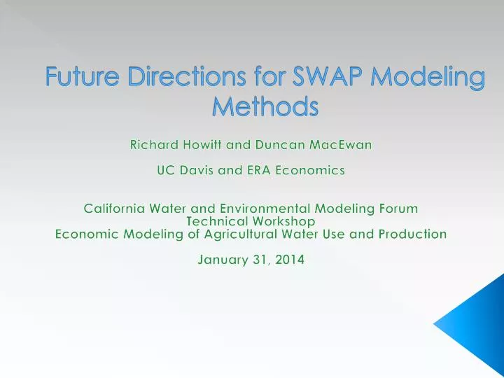
Future Directions for SWAP Modeling Methods. Richard Howitt and Duncan MacEwan UC Davis and ERA Economics California Water and Environmental Modeling Forum Technical Workshop Economic Modeling of Agricultural Water Use and Production January 31, 2014. Data Requirements.

E N D
Future Directions for SWAP Modeling Methods Richard Howitt and Duncan MacEwan UC Davis and ERA Economics California Water and Environmental Modeling Forum Technical Workshop Economic Modeling of Agricultural Water Use and Production January 31, 2014
Data Requirements • Significant effort with every project • Land use • Recent and reliable crop data • Water use • Disaggregation • Groundwater • Cost • Looking forward • Remote sensing? • Actively updated central database?
Remote Sensing and Agricultural Production: Land Use information • Land use (DWR, NAIP, NASS) • Digital elevation models (USGS) • Meteorological information (CIMIS) • County field surveys • Other survey data • Salinity With data from USDA Raster for Land Use for California http://www.nass.usda.gov/research/Cropland/cdorderform.htm
Pixel Classification Error Boundary Error
A brief history of PMP • Initial models and LP • Overspecialization, poor policy response • Positive Mathematical Programming • Howitt (1995) • Central Valley Production Model (CVPM) • PMP with limited input substitution • Statewide Agricultural Production Model (SWAP) • PMP with flexible CES production functions • Next iteration ??
A brief history of calibration • Positive Mathematical Programming • Calibration method: • 3 Steps • Economic first-order conditions hold exactly, elasticities are fit by OLS • Curvature in objective function from PMP cost functions (quadratic – CVPM; exponential SWAP) • Areas for refinement • Myopic calibration • First-order versus second-order calibration • Consistency with economic theory • Symmetry of policy response
Calibration developments • Howit (1995) • PMP first formalized • Various applications • CVPM Hatchett et al (1997) • SWAP Howitt et al (2012) • Heckelei (2002) • Critique of elasticity calibration, develop closed-form expression for fixed-proportions production function • Merel and Bucaram (2010) • Closed form solution for implied elasticities (non-myopic) • Merel, Simon, Yi (2011) • Fully calibrated (exact) decreasing returns to scale CES production function with single binding calibration constraint • Howitt and Merel (2014) • Review of state-of-the-art calibration methods • Garnache and Merel (2014) • Generalization of Merel, Simon, and Yi (2011) to multiple binding constraints
Current Research • Incorporate RTS exact calibration into SWAP • Understand tradeoffs and implications • Incorporating dynamic effects of crop rotations and stocks of groundwater • Validate and benchmark against other models and methods
Differences in Calibration of RTS models • LP stage I only provides consistent estimates of resource shadow values ( Lambda1) • Curvature in the objective function to calibrate crop specific inputs comes from the decreasing returns to scale (Delta) • Stage II– Least squares fit solves for parameters: Scale (alpha), Share(beta), RTS (delta) and Lambda2 (PMP cost) • Stage III Check the VMP conditions from stage II, and solve the unconstrained RTS problem
PMP-RTS Model • Differences • Delta is now greater than zero but less than one. • There is no non-linear PMP cost function • The PMP cost lambda2(i) is added to the cash costs Production Function:
Example of PMP v RTS • Calibrated output level = 865 tons • Note difference in curvature
Policy Value of RTS Specification • More precise supply elasticities • Second order calibration for policy response • Symmetry for crop acre increase or decrease • Crop area expansion • New crop introduction
Current Beta Version of SWAP-RTS • All crop inputs and outputs calibrate exactly • About half the regional crops pass the two Merel conditions. • Elasticities are minimum SSE estimates. • Calibration takes about half an hour, but once calibrated model solutions are fast. • Bio-physical priors can be a part of calibration- a test on water use efficiency worked well. • A small test version using OLS estimates over 5 years of data worked.