Download
1 / 34
340 likes | 346 Views
Recap: General Naïve Bayes. A general naïve Bayes model: Y: label to be predicted F 1 , …, F n : features of each instance. Y. F 1. F 2. F n. This slide deck courtesy of Dan Klein at UC Berkeley. Example Naïve Bayes Models. Bag-of-words for text

E N D
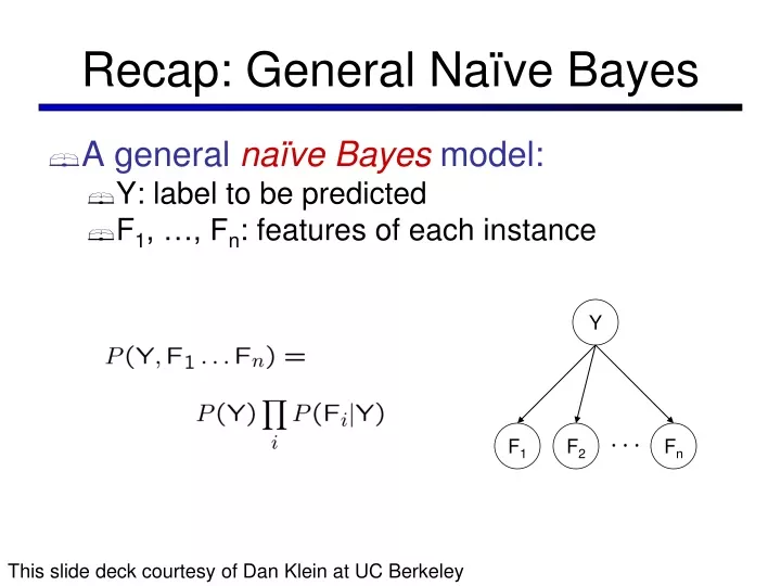
Recap: General Naïve Bayes • A general naïve Bayes model: • Y: label to be predicted • F1, …, Fn: features of each instance Y F1 F2 Fn This slide deck courtesy of Dan Klein at UC Berkeley
Example Naïve Bayes Models • Bag-of-words for text • One feature for every word position in the document • All features share the same conditional distributions • Maximum likelihood estimates: word frequencies, by label • Pixels for images • One feature for every pixel, indicating whether it is on (black) • Each pixel has a different conditional distribution • Maximum likelihood estimates: how often a pixel is on, by label Y Y W1 W2 Wn F0,0 F0,1 Fn,n
Naïve Bayes Training • Data: labeled instances, e.g. emails marked as spam/ham by a person • Divide into training, held-out, and test • Features are known for every training, held-out and test instance • Estimation: count feature values in the training set and normalize to get maximum likelihood estimates of probabilities • Smoothing (aka regularization): adjust estimates to account for unseen data Training Set Held-Out Set Test Set
Estimation: Smoothing • Problems with maximum likelihood estimates: • If I flip a coin once, and it’s heads, what’s the estimate for P(heads)? • What if I flip 10 times with 8 heads? • What if I flip 10M times with 8M heads? • Basic idea: • We have some prior expectation about parameters (here, the probability of heads) • Given little evidence, we should skew towards our prior • Given a lot of evidence, we should listen to the data
Estimation: Smoothing • Relative frequencies are the maximum likelihood estimates • In Bayesian statistics, we think of the parameters as just another random variable, with its own distribution ????
Recap: Laplace Smoothing • Laplace’s estimate (extended): • Pretend you saw every outcome k extra times • What’s Laplace with k = 0? • k is the strength of the prior • Laplace for conditionals: • Smooth each condition: • Can be derived by dividing H H T
Better: Linear Interpolation • Linear interpolation for conditional likelihoods • Idea: the conditional probability of a feature x given a label y should be close to the marginal probability of x • Example: A rare word like “interpolation” should be similarly rare in both ham and spam (a priori) • Procedure: Collect relative frequency estimates of both conditional and marginal, then average • Effect: Features have odds ratios closer to 1
Real NB: Smoothing • Odds ratios without smoothing: south-west : inf nation : inf morally : inf nicely : inf extent : inf ... screens : inf minute : inf guaranteed : inf $205.00 : inf delivery : inf ...
Real NB: Smoothing • Odds ratios after smoothing: helvetica : 11.4 seems : 10.8 group : 10.2 ago : 8.4 areas : 8.3 ... verdana : 28.8 Credit : 28.4 ORDER : 27.2 <FONT> : 26.9 money : 26.5 ... Do these make more sense?
Tuning on Held-Out Data • Now we’ve got two kinds of unknowns • Parameters: P(Fi|Y) and P(Y) • Hyperparameters, like the amount of smoothing to do: k, • Where to learn which unknowns • Learn parameters from training set • Can’t tune hyperparameters on training data (why?) • For each possible value of the hyperparameters, train and test on the held-out data • Choose the best value and do a final test on the test data Proportion of PML(x) in P(x|y)
Baselines • First task when classifying: get a baseline • Baselines are very simple “straw man” procedures • Help determine how hard the task is • Help know what a “good” accuracy is • Weak baseline: most frequent label classifier • Gives all test instances whatever label was most common in the training set • E.g. for spam filtering, might label everything as spam • Accuracy might be very high if the problem is skewed • When conducting real research, we usually use previous work as a (strong) baseline
Confidences from a Classifier • The confidence of a classifier: • Posterior of the most likely label • Represents how sure the classifier is of the classification • Any probabilistic model will have confidences • No guarantee confidence is correct • Calibration • Strong calibration: confidence predicts accuracy rate • Weak calibration: higher confidences mean higher accuracy • What’s the value of calibration?
Precision vs. Recall - • Let’s say we want to classify web pages as homepages or not • In a test set of 1K pages, there are 3 homepages • Our classifier says they are all non-homepages • 99.7 accuracy! • Need new measures for rare positive events • Precision: fraction of guessed positives which were actually positive • Recall: fraction of actual positives which were guessed as positive • Say we guess 5 homepages, of which 2 were actually homepages • Precision: 2 correct / 5 guessed = 0.4 • Recall: 2 correct / 3 true = 0.67 • Which is more important in customer support email automation? • Which is more important in airport face recognition? actual + guessed +
Precision vs. Recall • Precision/recall tradeoff • Often, you can trade off precision and recall • Only works well with weakly calibrated classifiers • To summarize the tradeoff: • Break-even point: precision value when p = r • F-measure: harmonic mean of p and r:
Naïve Bayes Summary • Bayes rule lets us do diagnostic queries with causal probabilities • The naïve Bayes assumption takes all features to be independent given the class label • We can build classifiers out of a naïve Bayes model using training data • Smoothing estimates is important in real systems • Confidences are useful when the classifier is calibrated
What to Do About Errors • Problem: there’s still spam in your inbox • Need more features – words aren’t enough! • Have you emailed the sender before? • Have 1K other people just gotten the same email? • Is the sending information consistent? • Is the email in ALL CAPS? • Do inline URLs point where they say they point? • Does the email address you by (your) name? • Naïve Bayes models can incorporate a variety of features, but tend to do best in homogeneous cases (e.g. all features are word occurrences)
Features • A feature is a function that signals a property of the input • Naïve Bayes: features are random variables & each value has conditional probabilities given the label. • Most classifiers: features are real-valued functions • Common special cases: • Indicator features take values 0 and 1 (or -1 and 1) • Count features return non-negative integers • Features are anything you can think of for which you can write code to evaluate on an input • Many are cheap, but some are expensive to compute • Can even be the output of another classifier or model • Domain knowledge goes here!
Feature Extractors • Features: anything you can compute about the input • A feature extractor maps inputs to feature vectors • Many classifiers take feature vectors as inputs • Feature vectors usually very sparse, use sparse encodings (i.e. only represent non-zero keys) Dear Sir. First, I must solicit your confidence in this transaction, this is by virture of its nature as being utterly confidencial and top secret. … W=dear : 1 W=sir : 1 W=this : 2 ... W=wish : 0 ... MISSPELLED : 2 YOUR_NAME : 1 ALL_CAPS : 0 NUM_URLS : 0 ...
Generative vs. Discriminative • Generative classifiers: • E.g. naïve Bayes • A causal model with evidence variables • Query model for causes given evidence • Discriminative classifiers: • No causal model, no Bayes rule, often no probabilities at all! • Try to predict the label Y directly from X • Robust, accurate with varied features • Loosely: mistake driven rather than model driven
Nearest-Neighbor Classification • Nearest neighbor for digits: • Take new image • Compare to all training images • Assign based on closest example • Encoding: image is vector of intensities: • What’s the similarity function? • Dot product of two images vectors? • Usually normalize vectors so ||x|| = 1 • min = 0 (when?), max = 1 (when?)
Clustering • Clustering systems: • Unsupervised learning • Detect patterns in unlabeled data • E.g. group emails or search results • E.g. find categories of customers • E.g. detect anomalous program executions • Useful when don’t know what you’re looking for • Requires data, but no labels • Often get gibberish
Clustering • Basic idea: group together similar instances • Example: 2D point patterns • What could “similar” mean? • One option: small (squared) Euclidean distance
K-Means • An iterative clustering algorithm • Pick K random points as cluster centers (means) • Alternate: • Assign data instances to closest mean • Assign each mean to the average of its assigned points • Stop when no points’ assignments change
K-Means as Optimization • Consider the total distance to the means: • Each iteration reduces phi • Two stages each iteration: • Update assignments: fix means c, change assignments a • Update means: fix assignments a, change means c means points assignments
Phase I: Update Assignments • For each point, re-assign to closest mean: • Can only decrease total distance phi!
Phase II: Update Means • Move each mean to the average of its assigned points: • Also can only decrease total distance… (Why?) • Fun fact: the point y with minimum squared Euclidean distance to a set of points {x} is their mean
Initialization • K-means is non-deterministic • Requires initial means • It does matter what you pick! • What can go wrong? • Various schemes for preventing this kind of thing: variance-based split / merge, initialization heuristics
K-Means Getting Stuck • A local optimum: Why doesn’t this work out like the earlier example, with the purple taking over half the blue?
K-Means Questions • Will K-means converge? • To a global optimum? • Will it always find the true patterns in the data? • If the patterns are very very clear? • Will it find something interesting? • Do people ever use it? • How many clusters to pick?
Agglomerative Clustering • Agglomerative clustering: • First merge very similar instances • Incrementally build larger clusters out of smaller clusters • Algorithm: • Maintain a set of clusters • Initially, each instance in its own cluster • Repeat: • Pick the two closest clusters • Merge them into a new cluster • Stop when there’s only one cluster left • Produces not one clustering, but a family of clusterings represented by a dendrogram
Agglomerative Clustering • How should we define “closest” for clusters with multiple elements? • Many options • Closest pair (single-link clustering) • Farthest pair (complete-link clustering) • Average of all pairs • Ward’s method (min variance, like k-means) • Different choices create different clustering behaviors
Clustering Application Top-level categories: supervised classification Story groupings: unsupervised clustering