Download

1 / 25
500 likes | 1.51k Views
Discrete Mathematics: Bayes’ Theorem and Expected Value and Variance. Section Summary. Bayes’ Theorem Bayesian Spam Filters Expected Value Linearity of Expectations Average-Case Complexity Geometric Distribution Independent Random Variables Variance. Motivation for Bayes ’ Theorem.

E N D
Discrete Mathematics: Bayes’ Theorem and Expected Value and Variance
Section Summary • Bayes’ Theorem • Bayesian Spam Filters • Expected Value • Linearity of Expectations • Average-Case Complexity • Geometric Distribution • Independent Random Variables • Variance
Motivation for Bayes’ Theorem • Bayes’ theorem allows us to use probability to answer questions such as the following: • Given that someone tests positive for having a particular disease, what is the probability that they actually do have the disease? • Given that someone tests negative for the disease, what is the probability that in fact they do have the disease? • Bayes’ theorem has applications to medicine, law, artificial intelligence, engineering, and many diverse other areas.
Bayes’ Theorem Bayes’ Theorem: suppose that E and F are events from a sample space S such that p(E)≠0 and p(F) ≠0. Then: Example: we have two boxes. The 1st box contains 2 green balls and 7 red balls. The 2nd contains 4 green balls and 3 red balls. Bob selects one of the boxes at random. Then he selects a ball from that box at random. If he has a red ball, what is the probability that he selected a ball from the 1st box. • Let E be the event that Bob has chosen a red ball and F be the event that Bob has chosen the 1st box. • By Bayes’ theorem the probability that Bob has picked the 1st box is:
Derivation of Bayes’ Theorem • Recall the definition of conditional probability p(E|F): • From this definition, it follows that:
Derivation of Bayes’ Theorem We know
Bayes’ Theorem in Medicine Example: suppose that one person in 100,000 has a particular disease. There is a test for the disease that gives a positive result99% of the time when given to someone with the disease. When given to someone without the disease, 99.5% of the time it gives a negative result. Find • The probability that a person who test positive has the disease. • The probability that a person who test negative does not have the disease. • Should someone who tests positive be worried?
Bayes’ Theorem in Medicine Solution-a: let Dbe the event that the person has the disease, and E be the event that this person tests positive. We need to compute p(D|E) from p(D), p(E|D), p( E |),p( ).
Bayes’ Theorem in Medicine Solution-b: what if the result is negative? The probability you have the disease if you test negative is It is extremely unlikely you have the disease if you test negative.
Bayesian Spam Filters • How do we develop a tool for determining whether an email is likely to be spam? • If we have an initial set B of spam messages and set G of non-spam messages. We can use this info along with Bayes’ law to predict the probability that an email message is spam. • We look at a particular word w, and count the number of times that it occurs in B and in G; nB(w) and nG(w). • Estimated probability that an email containing wis spam: p(w) = nB(w)/|B| • Estimated probability that an email containing wis not spam: q(w) = nG(w)/|G|
Bayesian Spam Filters • Let S be the event that the message is spam, and Ebe the event that the message contains the word w. • Assuming that it is equally likely that an arbitrary message is spam and is not spam, that is, p(S) = p(S) = ½. • If we have data on the frequency of spam messages, we can obtain a better estimate for p(w) and q(w). • r(w) estimates the probability that the message is spam. We can class the message as spam if r(w) is above a threshold.
Bayesian Spam Filters Example: we find that the word “Rolex” occurs in 250 out of 2000 spam messages and occurs in 5 out of 1000 non-spam messages. Estimate the probability that an incoming message is spam. Suppose our threshold for rejecting the email is 0.9. Solution: p(Rolex) =250/2000 =.0125 and q(Rolex) = 5/1000 = 0.005 We class the message as spam and reject the email.
Bayesian Spam Filters using Multiple Words • Accuracy can be improved by considering more than one word as evidence. • Consider the case where E1 and E2 denote the events that the message contains the words w1 and w2 respectively. • We make the simplifying assumption that the events are independent. And again we assume that p(S) = ½.
Bayesian Spam Filters using Multiple Words Example: we have 2000 spam messages and 1000non-spam messages. The word “stock” occurs 400times in the spam messages and 60 times in the non-spam. The word “undervalued” occurs in 200spam messages and 25 non-spam. Solution: p(stock) = 400/2000 = .2, q(stock) = 60/1000=.06, p(undervalued) = 200/2000 = .1, q(undervalued) = 25/1000 = .025 If our threshold is 0.9, we class the message as spam and reject it.
Bayesian Spam Filters using Multiple Words • In general, the more words we consider, the more accurate the spam filter. With the independence assumption if we consider k words: • We can further improve the filter by considering pairs of words as a single block or certain types of strings.
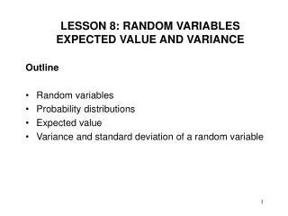
Expected Value Definition: the expected value(or expectationor mean) of the random variable X(s) on the sample space S is equal to Example: let X be the number that comes up when a fair dice is rolled. What is the expected value of X? Solution: random variable X takes the values 1, 2, 3, 4, 5, 6. Each has probability 1/6. It follows that
Expected Value Theorem: if X is a random variable and p(X = r) is the probability that X = r, so that then Theorem: the expected number of successes (with probability of p) when n mutually independent Bernoulli trials are performedis p= np. The next theorem tells us that expected values are linear, e.g., the expected value of the sum of random variables is the sum of their expected values. Theorem: if Xi, i = 1, 2, …, n with n a positive integer, are random variables on S, and if a and b are real numbers, then • E(X1 + X2 + …. + Xn) = E(X1 ) + E(X2) + … + E(Xn) • E(aX + b) = aE(X) + b.
Linearity of Expectations Hatcheck Problem: a new employee started a job checking hats, but forgot to put the claim check numbers on the hats. So, the n customers just receive a random hat from those remaining. What is the expected number of hat returned correctly? Solution: let X be the random variable that equals the number of people who receive the correct hat. Note that X = X1 + X2 + ∙∙∙ + Xn, where Xi = 1 if the ith person receives the hat and Xi = 0 otherwise. • Because it is equally likely that the checker returns any of the hats to the ith person, it follows that the probability that the ith person receives the correct hat is 1/n. Therefore, E(Xi) = 1 × p(Xi = 1) + 0 × p(Xi = 0) = 1 × 1/n + 0 = 1/n • By the linearity of expectations, it follows that: E(X )= E(X1) + E(X2) + ∙∙∙ + E(Xn) = n× 1/n= 1 Consequently, the average number of people who receive the correct hat is exactly one. Surprisingly, this answer remains the same no matter how many people have checked their hats!
Average-Case Computational Complexity Average-case computational complexity of an algorithm can be found by computing the expected value of a random variable. • Let the sample space of an experiment be the set of possible inputsaj, j = 1, 2, …, n and let the random variable X be the assignment to aj of the number of operations used by the algorithm when given ajas input. • Assign a probability p(aj) to each possible input value aj. • The expected value of X is the average-case computational complexity of the algorithm.
Average-Case Complexity of Linear Search What is the average-case complexity of linear search, described in Chapter 3, if the probability that x is in the list is p and it is equally likely that x is any of the n elements of the list? procedurelinearsearch (x: integer, a1, a2, …,an: distinct integers) i := 1 while (i≤n and x ≠ ai) i := i + 1 • ifi≤nthenlocation := i elselocation := 0 returnlocation
Average-Case Complexity of Linear Search Solution: there are n + 1possible types of input: one type for each of the n numbers on the list and one extra type for the numbers not on the list. • 2i + 1comparisons are needed if x equals the ith element of the list. • 2n + 2 comparisons are used if x is not on the list. The probability that x equals ai is p/nand the probability that x is not in the list is q = 1− p. The average-case complexity of the linear search is: E = 3p/n + 5p/n + … + (2n + 1)p/n + (2n + 2)q = (p/n)(3 + 5 + …. + (2n + 1)) + (2n + 2)q = (p/n)((n + 1)2− 1) + (2n + 2)q = p(n + 2) + (2n + 2)q • When x is guaranteed to be in the list, p = 1, q = 0, so that E = n + 2. • When p is ½ and q = ½, then E = (n + 2)/2 + n + 1 = (3n + 4) /2. • When p is ¾ and q = ¼ then E = (n + 2)/4 + (n + 1)/2 = (5n + 8) /4. • When x is guaranteed not to be in the list, p = 0 and q = 1, then E = 2n + 2.
The Geometric Distribution Definition: a random variable X has geometric distributionwith parameter p if p(X = k) = (1−p)k-1p for k = 1,2,3,…, where p is a real number with 0≤p≤1. Theorem: if random variable X has the geometric distribution with parameter p, then E(X) = 1/p. Example: suppose the probability that a coin comes up T is p. What is the expected number of flips until the coin comes up T? • The sample space is {T, HT, HHT, HHHT, HHHHT, …}. • Let X be the random variable equal to the number of flips in an element of the sample space; X(T) = 1, X(HT) = 2, X(HHT) = 3, etc. • p(T) = p , p(HT) = (1-p)p, p(HHT) = (1-p)2p , … ,therefore, E(X) = 1/p.
Independent Random Variables Definition: the random variables X and Y on a sample space S are independent if p(X = r1 and Y = r2) = p(X = r1) ×p(Y = r2). Theorem: if X and Y are independent variables on a sample space S, then E(XY) = E(X) E(Y)
Variance Deviation: the deviation of X at s ∊S is X(s) −E(X), the difference between the value of X and the mean of X. Definition: let X be a random variable on the sample space S. The variance of X, denoted by V(X) is That is V(X) is the weighted average of the square of the deviation of X. The standard deviation of X, denoted by σ(X) is defined to be Theorem: if X is a random variable on a sample space S, then V(X) = E(X2) −E(X)2 Corollary: if X is a random variable on a sample space S and E(X)=μ V(X) = E((X−μ)2)
Variance Example: whatis the variance of random variable X, where X(t) = 1 if a Bernoulli trial is a success and X(t) = 0 if it is a failure, where p is the probability of success and q is the probability of failure? Solution: because X takes only the values 0 and 1, it follows that X2(t) = X(t). Hence, Example: what is the variance of a random variable X, where X is the number that comes up when a fair dice is rolled? Solution: we have V(X) = E(X2) −E(X)2. In an earlier example, we saw that E(X) = 7/2. Note that E(X2) = 1/6(12 + 22 + 32 +42+ 52 + 62) = 91/6 We conclude that V(X) = E(X2) −E(X)2 = p−p2= p(1−p) = pq