Download
1 / 30
310 likes | 319 Views
Lecture 1: Course Overview and Introduction to Phasors. Prof. Niknejad. EECS 105: Course Overview. Phasors and Frequency Domain (2 weeks) Integrated Passives (R, C, L) (2 weeks) MOSFET Physics/Model (1 week) PN Junction / BJT Physics/Model (1.5 weeks) Single Stage Amplifiers (2 weeks)

E N D
Lecture 1: Course Overview and Introduction to Phasors Prof. Niknejad
EECS 105: Course Overview • Phasors and Frequency Domain (2 weeks) • Integrated Passives (R, C, L) (2 weeks) • MOSFET Physics/Model (1 week) • PN Junction / BJT Physics/Model (1.5 weeks) • Single Stage Amplifiers (2 weeks) • Feedback and Diff Amps (1 week) • Freq Resp of Single Stage Amps (1 week) • Multistage Amps (2.5 weeks) • Freq Resp of Multistage Amps (1 week) University of California, Berkeley
EECS 105 in the Grand Scheme • Example: Cell Phone University of California, Berkeley
MOS Cap Digital Gate Analog “Amp” Variable Capacitor PN Junction Transistors are Bricks • Transistors are the building blocks (bricks) of the modern electronic world: • Focus of course: • Understand device physics • Build analog circuits • Learn electronic prototyping and measurement • Learn simulations tools such as SPICE University of California, Berkeley
SPICE • SPICE = Simulation Program with ICEmphasis • Invented at Berkeley (released in 1972) • .DC: Find the DC operating point of a circuit • .TRAN: Solve the transient response of a circuit (solve a system of generally non-linear ordinary differential equations via adaptive time-step solver) • .AC: Find steady-state response of circuit to a sinusoidal excitation * Example netlist Q1 1 2 0 npnmod R1 1 3 1k Vdd 3 0 3v .tran 1u 100u SPICE stimulus response netlist University of California, Berkeley
BSIM • Transistors are complicated. Accurate sim requires 2D or 3D numerical sim (TCAD) to solve coupled PDEs (quantum effects, electromagnetics, etc) • This is slow … a circuit with one transistor will take hours to simulation • How do you simulate large circuits (100s-1000s of transistors)? • Use compact models. In EECS 105 we will derive the so called “level 1” model for a MOSFET. • The BSIM family of models are the industry standard models for circuit simulation of advanced process transistors. • BSIM = Berkeley Short Channel IGFET Model University of California, Berkeley
Berkeley… • A great place to study circuits, devices, and CAD! University of California, Berkeley
Review of LTI Systems • Since most periodic (non-periodic) signals can be decomposed into a summation (integration) of sinusoids via Fourier Series (Transform), the response of a LTI system to virtually any input is characterized by the frequency response of the system: Phase Shift Any linear circuit With L,C,R,M and dep. sources Amp Scale University of California, Berkeley
Example: Low Pass Filter (LPF) • Input signal: • We know that: Phase shift Amp shift University of California, Berkeley
LPF the “hard way” (cont.) • Plug the known form of the output into the equation and see if it can satisfy KVL and KCL • Since sine and cosine are linearly independent functions: IFF University of California, Berkeley
LPF: Solving for response… • Applying linear independence Phase Response: Amplitude Response: University of California, Berkeley
LPF Magnitude Response Passband of filter University of California, Berkeley
LPF Phase Response University of California, Berkeley
dB: Honor the inventor of the phone… • The LPF response quickly decays to zero • We can expand range by taking the log of the magnitude response • dB = deciBel (deci = 10) University of California, Berkeley
Why 20? Power! • Why multiply log by “20” rather than “10”? • Power is proportional to voltage squared: • At breakpoint: • Observe: slope of signal attenuation is 20 dB/decade in frequency University of California, Berkeley
Why introduce complex numbers? • They actually make things easier • One insightful derivation of • Consider a second order homogeneous DE • Since sine and cosine are linearly independent, any solution is a linear combination of the “fundamental” solutions University of California, Berkeley
Insight into Complex Exponential • But note that is also a solution! • That means: • To find the constants of prop, take derivative of this equation: • Now solve for the constants using both equations: University of California, Berkeley
The Rotating Complex Exponential • So the complex exponential is nothing but a point tracing out a unit circle on the complex plane: University of California, Berkeley
Magic: Turn Diff Eq into Algebraic Eq • Integration and differentiation are trivial with complex numbers: • Any ODE is now trivial algebraic manipulations … in fact, we’ll show that you don’t even need to directly derive the ODE by using phasors • The key is to observe that the current/voltage relation for any element can be derived for complex exponential excitation University of California, Berkeley
LTI System H Complex Exponential is Powerful • To find steady state response we can excite the system with a complex exponential • At any frequency, the system response is characterized by a single complex number H: • This is not surprising since a sinusoid is a sum of complex exponentials (and because of linearity!) • From this perspective, the complex exponential is even more fundamental Mag Response Phase Response University of California, Berkeley
LPF Example: The “soft way” • Let’s excite the system with a complex exp: use j to avoid confusion complex real Easy!!! University of California, Berkeley
Magnitude and Phase Response • The system is characterized by the complex function • The magnitude and phase response match our previous calculation: University of California, Berkeley
Why did it work? • The system is linear: • If we excite system with a sinusoid: • If we push the complex exp through the system first and take the real part of the output, then that’s the “real” sinusoidal response University of California, Berkeley
LTI System H LTI System H And yet another perspective… • Again, the system is linear: • To find the response to a sinusoid, we can find the response to and and sum the results: LTI System H University of California, Berkeley
Another persepctive (cont.) • Since the input is real, the output has to be real: • That means the second term is the conjugate of the first: • Therefore the output is: University of California, Berkeley
“Proof” for Linear Systems • For an arbitrary linear circuit (L,C,R,M, and dependent sources), decompose it into linear sub-operators, like multiplication by constants, time derivatives, or integrals: • For a complex exponential input x this simplifies to: University of California, Berkeley
“Proof” (cont.) • Notice that the output is also a complex exp times a complex number: • The amplitude of the output is the magnitude of the complex number and the phase of the output is the phase of the complex number University of California, Berkeley
Phasors • With our new confidence in complex numbers, we go full steam ahead and work directly with them … we can even drop the time factor since it will cancel out of the equations. • Excite system with a phasor: • Response will also be phasor: • For those with a Linear System background, we’re going to work in the frequency domain • This is the Laplace domain with University of California, Berkeley
+ _ Capacitor I-V Phasor Relation • Find the Phasor relation for current and voltage in a cap: University of California, Berkeley
+ _ Inductor I-V Phasor Relation • Find the Phasor relation for current and voltage in an inductor: University of California, Berkeley