Download
1 / 36
360 likes | 489 Views
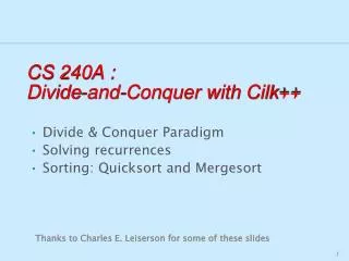
CS 240A : Divide-and-Conquer with Cilk ++. Divide & Conquer Paradigm Solving recurrences Sorting: Quicksort and Mergesort. Thanks to Charles E. Leiserson for some of these slides. Work and Span (Recap). T P = execution time on P processors. T 1 = work. T ∞ = span *.

E N D
CS 240A : Divide-and-Conquer with Cilk++ • Divide & Conquer Paradigm • Solving recurrences • Sorting: Quicksort and Mergesort Thanks to Charles E. Leiserson for some of these slides
Work and Span (Recap) TP = execution time on P processors T1 = work T∞= span* Speedup on p processors • T1/Tp Potential parallelism • T1/T∞
Sorting • Sorting is possibly the most frequently executed operation in computing! • Quicksort is the fastest sorting algorithm in practice with an average running time of O(N log N), (but O(N2) worst case performance) • Mergesort has worst case performance of O(N log N) for sorting N elements • Both based on the recursive divide-and-conquer paradigm
QUICKSORT • Basic Quicksort sorting an array S works as follows: • If the number of elements in S is 0 or 1, then return. • Pick any element vin S. Call this pivot. • Partition the set S-{v} into two disjoint groups: • S1 = {x S-{v} | x v} • S2 = {x S-{v} | x v} • Return quicksort(S1) followed by v followed by quicksort(S2)
QUICKSORT 14 13 45 56 34 31 32 21 78 Select Pivot 14 13 45 56 34 31 32 21 78
QUICKSORT 14 13 45 56 34 31 32 21 78 Partition around Pivot 56 13 31 21 45 34 32 14 78
QUICKSORT 56 13 31 21 45 34 32 14 78 Quicksort recursively 13 14 21 31 32 34 45 56 78 13 14 21 31 32 34 45 56 78
Parallelizing Quicksort • Serial Quicksort sorts an array S as follows: • If the number of elements in S is 0 or 1, then return. • Pick any element vin S. Call this pivot. • Partition the set S-{v} into two disjoint groups: • S1 = {x S-{v} | x v} • S2 = {x S-{v} | x v} • Return quicksort(S1)followed byv followed by quicksort(S2)
Parallel Quicksort (Basic) template <typename T> void qsort(T begin, T end) { if (begin != end) { T middle = partition( begin, end, bind2nd( less<typenameiterator_traits<T>::value_type>(), *begin ) ); cilk_spawnqsort(begin, middle); qsort(max(begin + 1, middle), end); cilk_sync; } } The second recursive call to qsort does not depend on the results of the first recursive call We have an opportunity to speed up the call by making both calls in parallel.
Performance • ./qsort 500000 -cilk_set_worker_count 1 >> 0.083 seconds • ./qsort 500000 -cilk_set_worker_count 16 >> 0.014 seconds • Speedup = T1/T16 = 0.083/0.014 = 5.93 • ./qsort 50000000 -cilk_set_worker_count 1 >> 10.57 seconds • ./qsort 50000000 -cilk_set_worker_count 16 >> 1.58 seconds • Speedup = T1/T16 = 10.57/1.58 = 6.67
workspan ws; ws.start(); sample_qsort(a, a + n); ws.stop(); ws.report(std::cout); Measure Work/Span Empirically • cilkscreen -w ./qsort 50000000 Work = 21593799861 Span = 1261403043 Burdened span = 1261600249 Parallelism = 17.1189 Burdened parallelism = 17.1162 #Spawn = 50000000 #Atomic instructions = 14 • cilkscreen -w ./qsort 500000 Work = 178835973 Span = 14378443 Burdened span = 14525767 Parallelism = 12.4378 Burdened parallelism = 12.3116 #Spawn = 500000 #Atomic instructions = 8
Analyzing Quicksort 56 13 31 21 45 34 32 14 78 Quicksort recursively 13 14 21 31 32 34 45 56 78 13 14 21 31 32 34 45 56 78 Assume we have a “great” partitioner that always generates two balanced sets
Analyzing Quicksort • Work: T1(n) = 2T1(n/2) + Θ(n) 2T1(n/2) = 4T1(n/4) + 2 Θ(n/2) …. …. n/2 T1(2) = n T1(1) + n/2 Θ(2) T1(n) = Θ(n lg n) • Span recurrence: T∞(n) = T∞(n/2) + Θ(n) Solves to T∞(n) = Θ(n) + Partitioning not parallel !
Parallelism: T1(n) = Θ(lg n) T∞(n) Analyzing Quicksort Not much ! • Indeed, partitioning (i.e., constructing the array S1 = {x S-{v} | x v})can be accomplished in parallel in time Θ(lg n) • Which gives a span T∞(n) = Θ(lg2n ) • And parallelismΘ(n/lg n) • Basic parallel qsort can be found in CLRS Way better !
The Master Method The Master Methodfor solving recurrences applies to recurrences of the form T(n) = aT(n/b) + f(n), where a ≥ 1, b > 1, and fis asymptotically positive. * Idea: Compare nlogba with f(n). * The unstated base case is T(n) = (1)for sufficiently small n.
Master Method — CASE 1 T(n) = a T(n/b) + f(n) nlogba≫ f(n) Specifically, f(n) = O(nlogba – ε) for some constant ε > 0 . Solution: T(n) = Θ(nlogba) . Eg matrix mult: a=8, b=2, f(n)=n2 T1(n)=Θ(n3)
Master Method — CASE 2 T(n) = a T(n/b) + f(n) nlogba≈ f(n) Specifically, f(n) = Θ(nlogbalgkn)for some constant k ≥ 0. Solution:T(n) = Θ(nlogbalgk+1n)) . Egqsort: a=2, b=2, k=0 T1(n)=Θ(n lg n)
Master Method — CASE 3 T(n) = a T(n/b) + f(n) nlogba≪ f(n) Specifically,f(n) = Ω(nlogba + ε)for some constant ε > 0,andf(n) satisfies the regularity conditionthat a f(n/b) ≤ c f(n)for some constant c < 1. Solution:T(n) = Θ(f(n)) . Eg: Span of qsort
Master Method Summary T(n) = a T(n/b) + f(n) CASE 1:f(n) = O(nlogba – ε), constant ε > 0 T(n) = Θ(nlogba) . CASE 2:f(n) = Θ(nlogba lgkn), constant k 0 T(n) = Θ(nlogba lgk+1n) . CASE 3:f(n) = Ω(nlogba + ε), constant ε > 0, and regularity condition T(n) = Θ(f(n)) .
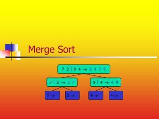
MERGESORT • Mergesort is an example of a recursive sorting algorithm. • It is based on the divide-and-conquer paradigm • It uses the merge operation as its fundamental component (which takes in two sorted sequencesandproduces a single sorted sequence) • Simulation of Mergesort • Drawback of mergesort: Not in-place (uses an extra temporary array)
Merging Two Sorted Arrays 3 12 19 46 4 14 21 23 template <typename T> void Merge(T *C, T *A, T *B, intna, intnb) { while (na>0 && nb>0) { if (*A <= *B) { *C++ = *A++; na--; } else { *C++ = *B++; nb--; } } while (na>0) { *C++ = *A++; na--; } while (nb>0) { *C++ = *B++; nb--; } } Time to merge n elements = Θ(n). 3 12 19 46 4 14 21 23
Parallel Merge Sort 3 4 12 14 19 21 33 46 3 12 19 46 4 14 21 33 3 19 12 46 4 33 14 21 A: input (unsorted) B: output (sorted) C: temporary template <typename T> void MergeSort(T *B, T *A, int n) { if (n==1) { B[0] = A[0]; } else { T* C = new T[n]; cilk_spawn MergeSort(C, A, n/2); MergeSort(C+n/2, A+n/2, n-n/2); cilk_sync; Merge(B, C, C+n/2, n/2, n-n/2); delete[] C; } } merge merge merge 19 3 12 46 33 4 21 14
Work of Merge Sort template <typename T> void MergeSort(T *B, T *A, int n) { if (n==1) { B[0] = A[0]; } else { T* C = new T[n]; cilk_spawn MergeSort(C, A, n/2); MergeSort(C+n/2, A+n/2, n-n/2); cilk_sync; Merge(B, C, C+n/2, n/2, n-n/2); delete[] C; } } CASE 2: nlogba = nlog22 = n f(n) = Θ(nlogbalg0n) 2T1(n/2) + Θ(n) Work:T1(n) = = Θ(n lg n)
Span of Merge Sort template <typename T> void MergeSort(T *B, T *A, int n) { if (n==1) { B[0] = A[0]; } else { T* C = new T[n]; cilk_spawn MergeSort(C, A, n/2); MergeSort(C+n/2, A+n/2, n-n/2); cilk_sync; Merge(B, C, C+n/2, n/2, n-n/2); delete[] C; } } CASE 3: nlogba = nlog21 = 1 f(n) = Θ(n) T∞(n/2) + Θ(n) Span:T∞(n) = = Θ(n)
Parallelism of Merge Sort Work: T1(n) = Θ(n lg n) PUNY! Span: T∞(n) = Θ(n) Parallelism: T1(n) = Θ(lg n) T∞(n) We need to parallelize the merge!
Parallel Merge ma = na/2 ≤ A[ma] ≥ A[ma] Recursive P_Merge Recursive P_Merge Binary Search ≤ A[ma] ≥ A[ma] mb mb-1 Throw away at least na/2 ≥ n/4 0 na A na ≥ nb B 0 nb Key Idea:If the total number of elements to be merged in the two arrays is n = na + nb, the total number of elements in the larger of the two recursive merges is at most (3/4)n .
Parallel Merge template <typename T> void P_Merge(T *C, T *A, T *B, intna, intnb) { if (na < nb) { P_Merge(C, B, A, nb, na); } else if (na==0) { return; } else { int ma = na/2; intmb = BinarySearch(A[ma], B, nb); C[ma+mb] = A[ma]; cilk_spawnP_Merge(C, A, B, ma, mb); P_Merge(C+ma+mb+1, A+ma+1, B+mb, na-ma-1, nb-mb); cilk_sync; } } Coarsen base cases for efficiency.
Span of Parallel Merge template <typename T> void P_Merge(T *C, T *A, T *B, int na, int nb) { if (na < nb) { ⋮ int mb = BinarySearch(A[ma], B, nb); C[ma+mb] = A[ma]; cilk_spawn P_Merge(C, A, B, ma, mb); P_Merge(C+ma+mb+1, A+ma+1, B+mb, na-ma-1, nb-mb); cilk_sync; } } CASE 2: nlogba = nlog4/31 = 1 f(n) = Θ(nlogba lg1n) T∞(3n/4) + Θ(lg n) Span:T∞(n) = = Θ(lg2n )
Work of Parallel Merge HAIRY! template <typename T> void P_Merge(T *C, T *A, T *B, int na, int nb) { if (na < nb) { ⋮ int mb = BinarySearch(A[ma], B, nb); C[ma+mb] = A[ma]; cilk_spawn P_Merge(C, A, B, ma, mb); P_Merge(C+ma+mb+1, A+ma+1, B+mb, na-ma-1, nb-mb); cilk_sync; } } T1(αn) + T1((1-α)n) + Θ(lg n), where 1/4 ≤ α≤ 3/4. Work:T1(n) = Claim:T1(n) = Θ(n).
Analysis of Work Recurrence Work: T1(n) = T1(αn) + T1((1-α)n) + Θ(lg n), where 1/4 ≤ α≤ 3/4. Substitution method: Inductive hypothesis is T1(k) ≤ c1k – c2lg k, wherec1,c2 > 0. Prove that the relation holds, and solve for c1 and c2. T1(n) = T1(n) + T1((1–)n) + (lg n) ≤ c1(n) – c2lg(n) + c1(1–)n – c2lg((1–)n) + (lg n)
Analysis of Work Recurrence Work: T1(n) = T1(αn) + T1((1-α)n) + Θ(lg n), where 1/4 ≤ α≤ 3/4. T1(n) = T1(n) + T1((1–)n) + (lg n) ≤ c1(n) – c2lg(n) + c1(1–)n – c2lg((1–)n) + (lg n)
Analysis of Work Recurrence Work: T1(n) = T1(αn) + T1((1-α)n) + Θ(lg n), where 1/4 ≤ α≤ 3/4. T1(n) = T1(n) + T1((1–)n) + Θ(lg n) ≤ c1(n) – c2lg(n) + c1(1–)n – c2lg((1–)n) + Θ(lg n) ≤ c1n – c2lg(n) – c2lg((1–)n) + Θ(lg n) ≤ c1n – c2 ( lg((1–)) + 2 lg n ) + Θ(lg n) ≤ c1n – c2 lg n – (c2(lg n + lg((1–))) – Θ(lg n)) ≤ c1n – c2 lg nby choosing c2 large enough. Choose c1 large enough to handle the base case.
Parallelism of P_Merge Parallelism: T1(n) = Θ(n/lg2n) T∞(n) Work: T1(n) = Θ(n) Span: T∞(n) = Θ(lg2n)
Parallel Merge Sort template <typename T> void P_MergeSort(T *B, T *A, int n) { if (n==1) { B[0] = A[0]; } else { T C[n]; cilk_spawnP_MergeSort(C, A, n/2); P_MergeSort(C+n/2, A+n/2, n-n/2); cilk_sync; P_Merge(B, C, C+n/2, n/2, n-n/2); } } CASE 2: nlogba = nlog22 = n f(n) = Θ(nlogba lg0n) 2T1(n/2) + Θ(n) Work:T1(n) = = Θ(n lg n)
Parallel Merge Sort template <typename T> void P_MergeSort(T *B, T *A, int n) { if (n==1) { B[0] = A[0]; } else { T C[n]; cilk_spawnP_MergeSort(C, A, n/2); P_MergeSort(C+n/2, A+n/2, n-n/2); cilk_sync; P_Merge(B, C, C+n/2, n/2, n-n/2); } } CASE 2: nlogba = nlog21 = 1 f(n) = Θ(nlogba lg2n) T∞(n/2) + Θ(lg2n) Span:T∞(n) = = Θ(lg3n)
Parallelism of P_MergeSort Work: T1(n) = Θ(n lg n) Span: T∞(n) = Θ(lg3n) Parallelism: T1(n) = Θ(n/lg2n) T∞(n)