Download
1 / 43
430 likes | 460 Views
"Explore the practical methods of decision tree learning for approximating discrete-valued functions through decision tree representation. Learn about top-down induction, statistical properties like information gain, and the significance of entropy in classification problems. Maria Simi provides insights and examples on how decision trees are used and created, making them robust to noisy data and ideal for various classification tasks such as equipment diagnosis and credit risk analysis. Gain a deeper understanding of entropy, information theory, and how to identify the best classifier through expected information gain calculation."

E N D
Decision tree learning Maria Simi, 2010/2011 Machine Learning, Tom Mitchell McGraw-Hill International Editions, 1997 (Cap 3).
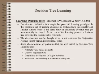
Inductive inference with decision trees • Decision Trees is one of the most widely used and practical methods of inductive inference • Features • Method for approximating discrete-valued functions (including boolean) • Learned functions are represented as decision trees (or if-then-else rules) • Expressive hypotheses space, including disjunction • Robust to noisy data Maria Simi
Decision tree representation (PlayTennis) Outlook=Sunny, Temp=Hot, Humidity=High, Wind=Strong No Maria Simi
Decision trees expressivity • Decision trees represent a disjunction of conjunctions on constraints on the value of attributes: (Outlook = Sunny Humidity = Normal) (Outlook = Overcast) (Outlook = Rain Wind = Weak) Maria Simi
Decision trees representation + Maria Simi
When to use Decision Trees • Problem characteristics: • Instances can be described by attribute value pairs • Target function is discrete valued • Disjunctive hypothesis may be required • Possibly noisy training data samples • Robust to errors in training data • Missing attribute values • Different classification problems: • Equipment or medical diagnosis • Credit risk analysis • Several tasks in natural language processing Maria Simi
Top-down induction of Decision Trees • ID3 (Quinlan, 1986) is a basic algorithm for learning DT's • Given a training set of examples, the algorithms for building DT performs search in the space of decision trees • The construction of the tree is top-down. The algorithm is greedy. • The fundamental question is “which attribute should be tested next? Which question gives us more information?” • Select the best attribute • A descendent node is then created for each possible value of this attribute and examples are partitioned according to this value • The process is repeated for each successor node until all the examples are classified correctly or there are no attributes left Maria Simi
Which attribute is the best classifier? • A statistical property called information gain, measures how well a given attribute separates the training examples • Information gain uses the notion of entropy, commonly used in information theory • Information gain = expected reduction of entropy Maria Simi
Entropy in binary classification • Entropy measures the impurity ofa collection of examples. It depends from the distribution of the random variable p. • S is a collection of training examples • p+ the proportion of positive examples in S • p– the proportion of negative examples in S Entropy (S) –p+log2p+ – p–log2p–[0 log20 = 0] Entropy ([14+, 0–]) = –14/14 log2 (14/14) – 0log2(0) = 0 Entropy ([9+, 5–]) = –9/14 log2 (9/14) – 5/14log2(5/14) = 0,94 Entropy ([7+, 7–]) = –7/14 log2 (7/14) –7/14log2(7/14) = = 1/2 +1/2 = 1 [log21/2 = –1] Note: the log of a number < 1 is negative, 0 p 1, 0 entropy 1 Maria Simi
Entropy Maria Simi
Entropy in general • Entropy measures the amount of information in a random variable H(X) = –p+log2p+ –p–log2p–X = {+, –} for binary classification [two-valued random variable] c c H(X) = – pilog2pi = pilog21/pi X = {i, …, c} i=1 i=1 for classification in c classes Example: rolling a die with 8, equally probable, sides 8 H(X) = – 1/8log21/8 = – log21/8 = log2 8= 3 i=1 Maria Simi
Entropy and information theory • Entropy specifies the number the average length (in bits) of the message needed to transmit the outcome of a random variable. This depends on the probability distribution. • Optimal length code assigns log2pbits to messages with probability p. Most probable messages get shorter codes. • Example: 8-sided [unbalanced] die 1 2 3 4 5 6 7 8 4/16 4/16 2/16 2/16 1/16 1/16 1/16 1/16 2 bits 2 bits 3 bits 3 bits 4bits 4bits 4bits 4bits E = (1/4 log2 4) 2 + (1/8 log2 8) 2 + (1/16 log2 16) 4 = 1+3/4+1 = 2,75 Maria Simi
|Sv| |S| Information gain as entropy reduction • Information gain is the expected reduction in entropy caused by partitioning the examples on an attribute. • The higher the information gain the more effective the attribute in classifying training data. • Expected reduction in entropy knowing A Gain(S, A) = Entropy(S)− Entropy(Sv) v Values(A) Values(A) possible values forA Sv subset ofS for whichA has valuev Maria Simi
Example: expected information gain • Let • Values(Wind) = {Weak, Strong} • S = [9+, 5−] • SWeak = [6+, 2−] • SStrong = [3+, 3−] • Information gain due to knowingWind: Gain(S, Wind) = Entropy(S) − 8/14 Entropy(SWeak) − 6/14 Entropy(SStrong) = 0,94 − 8/14 0,811 − 6/14 1,00 = 0,048 Maria Simi
Which attribute is the best classifier? Maria Simi
Example Maria Simi
First step: which attribute to test at the root? • Which attribute should be tested at the root? • Gain(S, Outlook) = 0.246 • Gain(S, Humidity) = 0.151 • Gain(S, Wind) = 0.084 • Gain(S, Temperature) = 0.029 • Outlook provides the best prediction for the target • Lets grow the tree: • add to the tree a successor for each possible value of Outlook • partition the training samples according to the value of Outlook Maria Simi
After first step Maria Simi
Second step • Working on Outlook=Sunny node: Gain(SSunny, Humidity) = 0.970 3/5 0.0 2/5 0.0 = 0.970 Gain(SSunny, Wind) = 0.970 2/5 1.0 3.5 0.918 = 0 .019 Gain(SSunny, Temp.) = 0.970 2/5 0.0 2/5 1.0 1/5 0.0 = 0.570 • Humidity provides the best prediction for the target • Lets grow the tree: • add to the tree a successor for each possible value of Humidity • partition the training samples according to the value of Humidity Maria Simi
{D1, D2, D8} No {D9, D11} Yes {D4, D5, D10} Yes {D6, D14} No Second and third steps Maria Simi
ID3: algorithm ID3(X, T, Attrs) X: training examples: T: target attribute (e.g. PlayTennis), Attrs: other attributes, initially all attributes Create Root node Ifall X's are +, returnRoot with class + If all X's are –, returnRoot with class– If Attrs is empty returnRoot with classmost common value of T in X else A best attribute; decision attribute for Root A For each possible value viof A: - add a new branch below Root, for test A = vi - Xi subset of X with A = vi - If Xiis emptythenadd a new leaf with class the most common value of T in X elseadd the subtree generated byID3(Xi, T, Attrs {A}) return Root Maria Simi
Search space in Decision Tree learning • The search space is made by partial decision trees • The algorithm is hill-climbing • The evaluation function is information gain • The hypotheses space is complete (represents all discrete-valued functions) • The search maintains a single current hypothesis • No backtracking; no guarantee of optimality • It uses all the available examples (not incremental) • May terminate earlier, accepting noisy classes Maria Simi
Inductive bias in decision tree learning • What is the inductive bias of DT learning? • Shorter trees are preferred over longer trees Not enough. This is the bias exhibited by a simple breadth first algorithm generating all DT's e selecting the shorter one • Prefer trees that place high information gain attributes close to the root • Note: DT's are not limited in representing all possible functions Maria Simi
Two kinds of biases • Preference or search biases (due to the search strategy) • ID3 searches a complete hypotheses space; the search strategy is incomplete • Restriction or language biases (due to the set of hypotheses expressible or considered) • Candidate-Elimination searches an incomplete hypotheses space; the search strategy is complete • A combination of biases in learning a linear combination of weighted features in board games. Maria Simi
Prefer shorter hypotheses: Occam's rasor • Why prefer shorter hypotheses? • Arguments in favor: • There are fewer short hypotheses than long ones • If a short hypothesis fits data unlikely to be a coincidence • Elegance and aesthetics • Arguments against: • Not every short hypothesis is a reasonable one. • Occam's razor:"The simplest explanation is usually the best one." • a principle usually (though incorrectly) attributed14th-century English logician and Franciscan friar, William of Ockham. • lexparsimoniae ("law of parsimony", "law of economy", or "law of succinctness") • The term razor refers to the act of shaving away unnecessary assumptions to get to the simplest explanation. Maria Simi
Issues in decision trees learning • Overfitting • Reduced error pruning • Rule post-pruning • Extensions • Continuous valued attributes • Alternative measures for selecting attributes • Handling training examples with missing attribute values • Handling attributes with different costs • Improving computational efficiency • Most of these improvements in C4.5 (Quinlan, 1993) Maria Simi
Overfitting: definition • Building trees that “adapt too much” to the training examples may lead to “overfitting”. • Consider error of hypothesis h over • training data: errorD(h) empirical error • entire distribution X of data: errorX(h) expected error • Hypothesis hoverfits training data if there is an alternative hypothesish' Hsuch that errorD(h) < errorD(h’) and errorX(h’) < errorX(h) i.e. h’ behaves better over unseen data Maria Simi
Example D15 Sunny Hot Normal Strong No Maria Simi
Overfitting in decision trees Outlook=Sunny, Temp=Hot, Humidity=Normal, Wind=Strong, PlayTennis=No New noisy example causes splitting of second leaf node. Maria Simi
Overfitting in decision tree learning Maria Simi
Avoid overfitting in Decision Trees • Two strategies: • Stop growing the tree earlier, before perfect classification • Allow the tree to overfit the data, and then post-prune the tree • Training and validation set • split the training in two parts (training and validation) and use validation to assess the utility of post-pruning • Reduced error pruning • Rule pruning • Other approaches • Use a statistical test to estimate effect of expanding or pruning • Minimum description length principle: uses a measure of complexity of encoding the DT and the examples, and halt growing the tree when this encoding size is minimal Maria Simi
Reduced-error pruning (Quinlan 1987) • Each node is a candidate for pruning • Pruning consists in removing a subtree rooted in a node: the node becomes a leaf and is assigned the most common classification • Nodes are removed only if the resulting tree performs no worse on the validation set. • Nodes are pruned iteratively: at each iteration the node whose removal most increases accuracy on the validation set is pruned. • Pruning stops when no pruning increases accuracy Maria Simi
Effect of reduced error pruning Maria Simi
Rule post-pruning • Create the decision tree from the training set • Convert the tree into an equivalent set of rules • Each path corresponds to a rule • Each node along a path corresponds to a pre-condition • Each leaf classification to the post-condition • Prune (generalize) each rule by removing those preconditions whose removal improves accuracy … • … over validation set • … over training with a pessimistic, statistically inspired, measure • Sort the rules in estimated order of accuracy, and consider them in sequence when classifying new instances Maria Simi
Converting to rules (Outlook=Sunny)(Humidity=High) ⇒ (PlayTennis=No) Maria Simi
Why converting to rules? • Each distinct path produces a different rule: a condition removal may be based on a local (contextual) criterion. Node pruning is global and affects all the rules • In rule form, tests are not ordered and there is no book-keeping involved when conditions (nodes) are removed • Converting to rules improves readability for humans Maria Simi
Dealing with continuous-valued attributes • So far discrete values for attributes and for outcome. • Given a continuous-valued attribute A, dynamically create a new attribute Ac Ac = True if A <c, False otherwise • How to determine threshold value c ? • Example. Temperature in the PlayTennisexample • Sort the examples according to Temperature Temperature 40 48 | 60 72 80 | 90 PlayTennisNo No 54 Yes Yes Yes 85 No • Determine candidate thresholds by averaging consecutive values where there is a change in classification: (48+60)/2=54 and (80+90)/2=85 • Evaluate candidate thresholds (attributes) according to information gain. The best is Temperature>54.The new attribute competes with the other ones Maria Simi
Problems with information gain • Natural bias of information gain: it favours attributes with many possible values. • Consider the attribute Datein thePlayTennisexample. • Date would have the highest information gain since it perfectly separates the training data. • It would be selected at the root resulting in a very broad tree • Very good on the training, this tree would perform poorly in predicting unknown instances. Overfitting. • The problem is that the partition is too specific, too many small classes are generated. • We need to look at alternative measures … Maria Simi
An alternative measure: gain ratio c |Si | |Si | SplitInformation(S, A) − log2i=1 |S | |S | • Siare the sets obtained by partitioning on value i ofA • SplitInformation measures the entropy of S with respect to the values of A. The more uniformly dispersed the data the higher it is. Gain(S, A) GainRatio(S, A) SplitInformation(S, A) • GainRatio penalizes attributes that split examples in many small classes such asDate. Let |S |=n, Date splits examples inn classes • SplitInformation(S, Date)= −[(1/nlog2 1/n)+…+ (1/nlog2 1/n)]= −log21/n =log2n • Compare with A, which splits data in two even classes: • SplitInformation(S, A)= − [(1/2 log21/2)+ (1/2 log21/2) ]= − [− 1/2 −1/2]=1 Maria Simi
Adjusting gain-ratio • Problem: SplitInformation(S, A) can be zero or very small when|Si | ≈ |S| for some value i • To mitigate this effect, the following heuristics has been used: • computeGainfor each attribute • applyGainRatioonly to attributes with Gainabove average • Other measures have been proposed: • Distance-based metric [Lopez-De Mantaras, 1991] on the partitions of data • Each partition (induced by an attribute) is evaluated according to the distance to the partition that perfectly classifies the data. • The partition closest to the ideal partition is chosen Maria Simi
Handling incomplete training data • How to cope with the problem that the value of some attribute may be missing? • Example: Blood-Test-Result in a medical diagnosis problem • The strategy: use other examples to guess attribute • Assign the value that is most common among the training examples at the node • Assign a probability to each value, based on frequencies, and assign values to missing attribute, according to this probability distribution • Missing values in new instances to be classified are treated accordingly, and the most probable classification is chosen (C4.5) Maria Simi
Handling attributes with different costs • Instance attributes may have an associated cost: we would prefer decision trees that use low-cost attributes • ID3 can be modified to take into account costs: • Tan and Schlimmer (1990) Gain2(S, A) Cost(S, A) • Nunez (1988) 2Gain(S, A) 1 (Cost(A) + 1)w w ∈[0,1] Maria Simi
References • Machine Learning, Tom Mitchell, Mc Graw-Hill International Editions, 1997 (Cap 3). Maria Simi