Download
1 / 36
370 likes | 451 Views
Decision Tree Learning. Seong-Bae Park. Main Idea. Classification by Partitioning Example Space Goal : Approximating discrete-valued target functions Appropriate Problems Examples are represented by attribute-value pairs. The target function has discrete output value.

E N D
Decision Tree Learning Seong-Bae Park
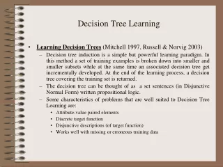
Main Idea • Classification by Partitioning Example Space • Goal : Approximating discrete-valued target functions • Appropriate Problems • Examples are represented by attribute-value pairs. • The target function has discrete output value. • Disjunctive description may be required. • The training data may contain missing attribute values. SNU Center for Bioinformation Technology (CBIT)
Example Space Yes (Outlook = Overcast) No (Outlook = Sunny & Humidity = High) Yes (Outlook = Sunny & Humidity = Normal) Yes (Outlook = Rain & Wind = Weak) No (Outlook = Rain & Wind = Strong) SNU Center for Bioinformation Technology (CBIT)
Decision Tree Representation Outlook Rain Sunny Overcast Humidity Wind YES High Normal NO YES NO YES SNU Center for Bioinformation Technology (CBIT)
Basic Decision Tree Learning • Which Attribute is Best? • Select the attribute that is most useful for classifying examples. • Quantitative Measure • Information Gain • For Attribute A, relative to a collection of data D • Expected Reduction of Entropy SNU Center for Bioinformation Technology (CBIT)
1.0 Entropy(S) 0.0 1.0 Entropy • Impurity of an Arbitrary Collection of Examples • Minimum number of bits of information needed to encode the classification of an arbitrary member of D SNU Center for Bioinformation Technology (CBIT)
Constructing Decision Tree SNU Center for Bioinformation Technology (CBIT)
Example : Play Tennis (1) • Entropy of D SNU Center for Bioinformation Technology (CBIT)
[9+,5-] : E = 0.940 Wind Weak Strong [6+,2-] : E = 0.811 [3+,3-] : E = 1.0 Example : Play Tennis (2) • Attribute Wind • D = [9+,5-] • Dweak = [6+,2-] • Dstrong=[3+,3-] SNU Center for Bioinformation Technology (CBIT)
[9+,5-] : E = 0.940 Humidity High Normal [3+,4-] : E = 0.985 [6+,1-] : E = 0.592 Example : Play Tennis (3) • Attribute Humidity • Dhigh = [3+,4-] • Dnormal=[6+,1-] SNU Center for Bioinformation Technology (CBIT)
[9+,5-] : E = 0.940 Outlook Sunny Rain Overcast [2+,3-] : (D1, D2, D8, D9, D11) [4+,0-] : (D3, D7, D12, D13) YES [3+,2-] : (D4, D5, D6, D10, D14) Example : Play Tennis (4) • Best Attribute? • Gain(D, Outlook) = 0.246 • Gain(D, Humidity) = 0.151 • Gain(D, Wind) = 0.048 • Gain(D, Temperature) = 0.029 SNU Center for Bioinformation Technology (CBIT)
Example : Play Tennis (5) • Entropy Dsunny SNU Center for Bioinformation Technology (CBIT)
[2+,3-] : E = 0.971 Wind Weak Strong [1+,2-] : E = 0.918 [1+,1-] : E = 1.0 Example : Play Tennis (6) • Attribute Wind • Dweak = [1+,2-] • Dstrong=[1+,1-] SNU Center for Bioinformation Technology (CBIT)
[2+,3-] : E = 0.971 Humidity High Normal [0+,3-] : E = 0.00 [2+,0-] : E = 0.00 Example : Play Tennis (7) • Attribute Humidity • Dhigh = [0+,3-] • Dnormal=[2+,0-] SNU Center for Bioinformation Technology (CBIT)
Example : Play Tennis (8) • Best Attribute? • Gain(D, Humidity) = 0.971 • Gain(D, Wind) = 0.020 • Gain(D, Temperature) = 0.571 [9+,5-] : E = 0.940 Outlook Sunny Overcast Rain Humidity YES [3+,2-] : (D4, D5, D6, D10, D14) High Normal NO YES SNU Center for Bioinformation Technology (CBIT)
Example : Play Tennis (9) • Entropy Drain SNU Center for Bioinformation Technology (CBIT)
[3+,2-] : E = 0.971 Wind Weak Strong [3+,0-] : E = 0.00 [0+,2-] : E = 0.00 Example : Play Tennis (10) • Attribute Wind • Dweak = [3+,0-] • Dstrong=[0+,2-] SNU Center for Bioinformation Technology (CBIT)
[2+,3-] : E = 0.971 Humidity High Normal [1+,1-] : E = 1.00 [2+,1-] : E = 0.918 Example : Play Tennis (11) • Attribute Humidity • Dhigh = [1+,1-] • Dnormal=[2+,1-] SNU Center for Bioinformation Technology (CBIT)
Outlook Rain Sunny Overcast Humidity Wind YES High Normal NO YES NO YES Example : Play Tennis (12) • Best Attribute? • Gain(D, Humidity) = 0.020 • Gain(D, Wind) = 0.971 • Gain(D, Temperature) = 0.020 SNU Center for Bioinformation Technology (CBIT)
Avoiding Overfitting Data • Data Overfitting • Consider the following: (Outlook = Sunny & Humidity = Normal & PlayTennis = No) • Wrong Decision Tree Prediction • (Outlook = Sunny & Humidity = Normal) Yes • What if we prune ‘Humidity’ node? • When (outlook = Sunny), PlayTennis No • Can be correctly predicted. SNU Center for Bioinformation Technology (CBIT)
Outlook Rain Sunny Overcast Wind (2+,3-) NO YES NO YES Avoiding Overfitting Data (2) SNU Center for Bioinformation Technology (CBIT)
Avoiding Overfitting Data (3) • Definition • Given a hypothesis space H, a hypothesis hH is said to overfit the data if there exists some alternative hypothesis h’ H, such that h has smaller error than h’ over the training examples, but h’ has a smaller error than h over entire distribution of instances. • Occam’s Razor • Prefer the simplest hypothesis that fits the data. SNU Center for Bioinformation Technology (CBIT)
Avoiding Overfitting Data (4) SNU Center for Bioinformation Technology (CBIT)
Avoiding Overfitting Data (5) • Solutions 1. Partition examples into training, test, and validation set. 2. Use all data for training, but apply a statistical test to estimate whether expanding (or pruning) a particular node is likely to produce an improvement beyond the training set. 3. Use an explicit measure of the complexity for encoding the training examples and the decision tree, halting growth of the tree when this encoding is minimized. SNU Center for Bioinformation Technology (CBIT)
Decision Tree Tool: C4.5 • Reference: • Ross Quinlan, C4.5: Programs for Machine Learning, Morgan Kaufmann Publishers, 1993. • Source Code Download • http://www.cse.unsw.edu.au/~quinlan/ SNU Center for Bioinformation Technology (CBIT)
How to Use C4.5 (1) • First Step • Define the classes and attributes • .names file: labor-neg.names Good, bad. Duration: continuous. Wage increase first year: continuous. Wage increase second year: continuous. Wage increase third year: continuous. Cost of living adjustment: none, tcf, tc. Working hours: continuous Pension: none, ret_allw, empl_contr. Standby pay: continuous. Shift differential: continuous. Education allowance: yes, no. Statutory holidays: continuous. Vacation: below average, average, generous. Longterm disability assistance: yes, no. Contribution to dental plan: none, half, full. Bereavement assistance: yes, no. Contribution to health plan: none, half, full. SNU Center for Bioinformation Technology (CBIT)
How to Use C4.5 (2) • Second Step • Provide information on the individual cases • .data file: labor-neg.data • Example: 1, 2.0, ?, ?, none, 38, none, ?, ?, yes, 11, average, no, none, no, none, bad. 2, 4.0, 5.0, ?, tcf, 35, ?, 13, 5, ?, 15, generous, ?, ?, ?, ?, good. 2, 4.3, 4.4, ?, ?, 38, ?, ?, 4, ?, 12, generous, ?, full, ?, full, good. • ?: unknown or inapplicable values • .test file: labor-neg.test SNU Center for Bioinformation Technology (CBIT)
How to Use C4.5 (3) • Third Step • Run C4.5 • Command: • c4.5 –f labor-neg –u SNU Center for Bioinformation Technology (CBIT)
Example: Learning to Classify Text • Representing Document in a Vector • Dimension = |Vocabulary| • Weight of a term tjappeared in the document di • tfij: the frequency of tj in di • N: the number of total documents • n: the number of documents where tj occurs at least once SNU Center for Bioinformation Technology (CBIT)
HPV Sequence Database • The HPV Sequence Database • Los Alamos National Laboratory • http:// <definition> Human papillomavirus type 80 E6, E7, E1, E2, E4, L2, and L1 genes. </definition> <source> Human papillomavirus type 80. </source> <comment> The DNA genome of HPV80 (HPV15-related) was isolated from histologically normal skin, cloned, and sequenced. HPV80 is most similar to HPV15, and falls within one of the two major branches of the B1 or Cutaneous/EV clade. The E7, E1, and E4 orfs, as well as the URR, of HPV15 and HPV80 share sequence similarities higher than 90%, while in the usually more conservative L1 orf the nucleotide similarity is only 87%. A detailed comparative sequence analysis of HPV80 revealed features characteristic of a truly cutaneous HPV type [362]. Notice in the alignment below that HPV80 compares closely to the cutaneous types HPV15 and HPV49 in the important E7 functional regions CR1, pRb binding site, and CR2. HPV 80 is distinctly different from the high-risk mucosal viruses represented by HPV16. The locus as defined by GenBank is HPVY15176. </comment> SNU Center for Bioinformation Technology (CBIT)
Representing Document • Stemming and stopword list • Porter’s Stemmer • Remove numeric expression and prepositions • |Vocabulary| = 1434 • HPV80 Description 42: 0.445260 145: 3.367296 205: 3.367296 211: 0.476924 215: 1.352393 296: 2.990987 314: 1.227230 388: 0.090151 521: 2.451005 529: 2.114533 530: 1.421386 544: 0.764606 579: 1.575536 580: 2.674149 608: 2.961831 763: 1.495494 772: 1.863218 780: 0.034783 851: 2.114533 987: 1.683134 1004: 2.674149 1076: 2.268646 1093: 0.764606 1148: 1.421386 1187: 2.961831 1201: 2.774846 1206: 1.227230 1211: 1.662548 1377: 1.757858 1404: 0.841567 SNU Center for Bioinformation Technology (CBIT)
Classify HPVs • Goal • Classify the Risk Types of HPVs related with cervical cancer • Class: High, Low • Training Set: (Virology, Prentice Hall, 1994) • HPV6: Low • HPV11: Low • HPV16: High • HPV18: High • HPV31: High • HPV33: High • HPV45: High SNU Center for Bioinformation Technology (CBIT)
Classifying All HPVs C4.5 [release 8] decision tree generator ---------------------------------------- Options: File stem <hpv> Trees evaluated on unseen cases Read 7 cases (1434 attributes) from hpv.data Decision Tree: W546 > 1.86322 : 1 (5.0) W546 <= 1.86322 : | W432 > 0 : 1 (3.0) | W432 <= 0 : | | W785 > 0 : 1 (3.0/1.0) | | W785 <= 0 : | | | W511 <= 0 : | | | | W142 <= 1.49549 : 0 (40.0) | | | | W142 > 1.49549 : 1 (3.0/1.0) | | | W511 > 0 : | | | | W544 <= 0 : 1 (2.0) | | | | W544 > 0 : 0 (2.0) Evaluation on training data (7 items): Before Pruning After Pruning ---------------- --------------------------- Size Errors Size Errors Estimate 13 0( 0.0%) 13 0( 0.0%) (0.0%) << Evaluation on test data (76 items): Before Pruning After Pruning ---------------- --------------------------- Size Errors Size Errors Estimate 13 2(2.6%) 13 2(2.6%) (13.3%) << SNU Center for Bioinformation Technology (CBIT)
Summary • Decision Tree provides a practical method for concept learning and discrete-valued functions. • ID3 searches a complete hypothesis space. • Overfitting is an important issue in decision tree learning. SNU Center for Bioinformation Technology (CBIT)