Download
1 / 17
170 likes | 261 Views
Wavelet-based Nonparametric Modeling of Hierarchical Functions in Colon Carcinogenesis. Jeffrey S. Morris M.D. Anderson Cancer Center Joint work with Marina Vannucci, Philip J. Brown, and Raymond J. Carroll. 1. Introduction

E N D
Wavelet-based Nonparametric Modeling of Hierarchical Functions in Colon Carcinogenesis Jeffrey S. Morris M.D. Anderson Cancer Center Joint work with Marina Vannucci, Philip J. Brown, and Raymond J. Carroll
1. Introduction • In this work, we have developed a new method to model hierarchical functional data, which is a special type of correlated longitudinal data. • Modeling of the longitudinal profiles is done nonparametrically, with regularization done via wavelet shrinkage. • We model all the data simultaneously using a single hierarchical model, an approach that naturally adjusts for imbalance in the design and accounts for the correlation structure among the individual profiles. • Our method yields estimates and posterior samples for mean as well as individual-level profiles, plus interprofile covariance parameters. • This work was motivated by and applied to a data set from a colon carcinogenesis study.
2. Biological Background of Application: Cellular Structure of the Colon • Colon cells grow within crypts, fingerlike structures that grow into the wall of the colon. • Individual colon cells are generated from stem cells at the bottom of the crypt, and move up the crypt as they mature. • This means a cell’s relative depth within the crypt is related to its age and stage in the cell cycle, and as a result it is important to model biological processes in the colon as functions of relative cell position. • Define t = relative cell position, t (0,1) 0 = bottom of crypt, 1 = top of crypt
3. The Colon Carcinogenesis Study Previous studies have demonstrated that diets high in fish oil fats are protective against colon cancer compared with corn oil diets, but the biological mechanisms behind this effect are not known. One hypothesis is that the body is not effectively repairing damage to cells’ DNA caused by exposure to a carcinogen. This hypothesis was investigated in the following rat colon carcinogenesis experiment. The Data: • Rats were fed one of two diets (fish/corn oil), exposed to carcinogen, then euthanized at one of 5 times after exposure (0,3,6,9,12 hr). Their colons were removed and stained to quantify the levels of a DNA repair enzyme. • 3 rats in each of the 10 diet time groups. • 25 crypts sampled from each rat • Response quantified on equally spaced grid (~300) along left side of crypt • Hierarchical functional data: Longitudinal profile for each crypt, with crypts nested within rats, and rats further nested within treatment.
4. The Colon Carcinogenesis Study • Some questions of interest from these data: • Do fish oil rats have more DNA repair enzyme than corn oil rats? Does this relationship depend on time since carcinogen exposure and/or depth within the crypt? • Does DNA repair enzyme activity vary w.r.t. depth within crypt? • Where is the majority of variability in DNA repair expression, between rats, between crypts, or within crypts? • Are there any rats and/or crypts with unusual DNA repair profiles? • We set out to answer questions like these using a single unified model for all the data.
5. Hierarchical Functional Model • Following is a model we can use to think about our data: • MODEL (1): If we were willing to place parametric assumptions on g functions, model (1) simplifies to standard mixed model. • Yabc= response vector for crypt c, rat b of treatment group aon grid t • g·(t) = true crypt, rat, or treatment-level profiles • eabc= measurement error (iid normals) • abc(t), ab(t) = crypt/rat level error processes; mean 0 with covariances 1(t1,t2) and 2 (t1,t2) 6 of the 750 observed crypt profiles of DNA repair enzyme • For our data, we need nonparametric method, that can handle spatially heterogeneous functions. • In single function setting, wavelet regression effective for modeling functions like these.
6. Overview of Wavelets • Useful Properties of Wavelets • Parsimonious representation: Many functions can be represented almost perfectly with just ~5% of the wavelet coefficients. • Fast Computation: O(n) algorithm (DWT) available to compute set of n wavelet coefficients from n data points (IDWT to do inverse transformation). • Linear Transformation: Switching between data and wavelet spaces involves linear transformation, which preserves hierarchical relationships between profiles in our model. • Whitening property: Wavelet coeffs. much less correlated than original data. Wavelets are orthonormal basis functions that can be used to parsimoniously represent other functions. Daubechies Basis Function
7. Overview of Method • Implementation of our method fundamentally involves three steps: • Perform a DWT on the response vector for each crypt, yabc, to obtain the corresponding set of empirical wavelet coefficients, dabc. The wavelet coefficients are double-indexed by j, corresponding to the scale, and k the location. • Fit a Bayesian multilevel hierarchical model to these empirical wavelet coefficients, yielding posterior samples of the true wavelet coefficients which correspond to the treatment, rat, and crypt-level profiles, plus the covariance parameters at these levels. - This model incorporates a shrinkage prior at the top level of the hierarchy, that uses nonlinear shrinkage to perform smoothing, or regularization, in the nonparametric estimation of the profiles. • Posterior samples of any treatment, rat, or crypt-level profiles of interest can be obtained by applying IDWTs to the corresponding of true wavelet coefficient estimates. These samples can be used for estimation or Bayesian inference.
8. Wavelet Space Model • Notes on Wavelet Space Model • All quantities in data space model (1) obtainable using IDWT on quantities in wavelet space model (2). • Although independence assumed in wavelet space, model (2) accommodates varying degrees of autocorrelation in data space. • Measurement error variance in wavelet space,2e, the same as in data space. Plug-in estimate used as in Donoho&Johnstone(1994) • For Bayesian inference, vague proper priors placed on variance components, and shrinkage prior placed on top level coeffs. aj,k. • Assuming the wavelet coefficients are independent, we specify a (scalar) hierarchical model for the empirical wavelet coefficients. • MODEL 2 • abcj,k,abj,k, aj,k: true wavelet coefficients at crypt, rat, trt levels • 22,j, 21,j, 2e: variance components between rats, between crypts, and within crypts at wavelet scale j
9. Shrinkage Prior One property of the wavelet transform is that it tends to distribute any noise equally among all the wavelet coefficients. Given the parsimony property, this means that a majority of the coefficients will be small, and consist almost entirely of noise, while a small proportion will be large and contain primarily signal. In order to perform regularization, we would like to shrink the wavelet coefficients towards zero in a nonlinear fashion so that, if it is large, we leave it alone since we think it is signal. The smaller it is, the more we would like to shrink it, since we then think it is noise. This type of nonlinear shrinkage results in denoised, or regularized, estimators. This nonlinear shrinkage is achieved in our model via a prior on aj,k.that is a mixture of point mass at zero and a normal, which we call a shrinkage prior. Shrinkage Prior: pj= expected proportion of ‘nonzero’ wavelet coefficients at wavelet scale j. 2j = variance of ‘nonzero’ wavelet coefficients at wavelet scale j.
10. Fitting the Model • The shrinkage prior requires us to use an MCMC to fit model (2). • We initially integrate out the random effects to improve convergence. • STEPS: • If rat/crypt level profiles are desired, we proceed to sample random effects: • Inverse Discrete Wavelet Transforms are applied to the sets of wavelet coefficients to get the corresponding profiles
11. Application: Results 0h 3h 6h 9h 12h • Key Results: • More DNA Repair at top of crypts, which is where tumors form. • No diet/time effect evident through 9h • Strange results at 12h • - Fish>Corn at top • - Caused by outlier? Fish Oil Corn Oil Estimated diet/time profiles of DNA Repair Enzyme with 90% pointwise posterior credible bounds.
12. Application: Results • Effect consistent across rats – 12h effect not driven by outlier • Relative Variability: 79% between crypts, 20% between rats, 1% within crypts: Implies importance of sampling lots of crypts • Variance components at wavelet resolution levels reveal insights about nature of profiles: - Rat profiles more smooth - Crypt profiles characterized by peaks of width ~20 pixels (peaks = individual cells?) Fish Oil Corn Oil Estimated rat profiles for all rats at 12 hour time point, with 90% posterior credible intervals. The dashed lines are naïve estimates obtained by simply averaging the data over crypts.
13. Sensitivity Analysis • Uninformative priors used everywhere, except shrinkage hyperparameters p and T2, • Sensitivity analysis reveals this prior affects the smoothness of the underlying estimator, but not the substantive results. • Thus, these parameters are essentially smoothing parameters, or more accurately, regularization parameters. Estimated profiles at 12 hour time point, with 90% posterior credible intervals, using different values for the shrinkage hyperparameters p and T2
14. Conclusions • New method to fit hierarchical longitudinal data, yielding: • Nonparametric regularized estimates of profiles at mean, individual and subsampling levels • Covariance parameter estimates, from which correlation matrices at various hierarchical levels can be constructed. • Posterior samples from MCMC enable various Bayesian inferences to be done. • All done with unified, ‘nonparametric’ model that appropriately adjusts for imbalance & correlation. • Wavelets allow use of simpler covariance structures, work well for spatially heterogeneous functions, and give multiresolution analysis. • Our method can be generalized to more complex covariance structures, effectively yielding a ‘nonparametric’ functional mixed model.
15. How does the nonlinear shrinkage work? Consider the shrinkage estimator for one of the wavelet coefficients, which can be seen to be a product of the (unshrunken) MLE and a shrinkage factor h. This shrinkage factor depends on the hyperparameters (pjand 2j) and Z, which measures the distance between the MLE and zero in units of its standard deviation This shrinkage factor has two parts: one that performs linear shrinkage, which applies equally no matter what the magnitude of the data, and one that performs nonlinear shrinkage, which shrinks more for data closer to zero. Note that the nonlinear shrinkage involves the posterior odds that the coefficient aj,k is nonzero.
16. How does the nonlinear shrinkage work? Shrinkage as function of Z=size of coefficient for p=0.50 and p=0.10, and various choices of T2. • Notes about shrinkage curves • Coefficients close to zero are shrunken the most. • Making pj smaller causes more shrinkage of coefficients, and thus more smoothing of features at wavelet scale j. • Making T2jtoo small results in much shrinkage, even for large coefficients. • Making T2jtoo large causes a Lindley’s paradox-type effect, which is manifested in steep shrinkage curves.