Download
1 / 65
670 likes | 783 Views
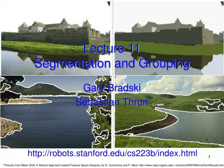
Lecture 11 Segmentation and Grouping. Gary Bradski Sebastian Thrun. *. http://robots.stanford.edu/cs223b/index.html. * Pictures from Mean Shift: A Robust Approach toward Feature Space Analysis, by D. Comaniciu and P. Meer http://www.caip.rutgers.edu/~comanici/MSPAMI/msPamiResults.html.

E N D
Lecture 11Segmentation and Grouping Gary Bradski Sebastian Thrun * http://robots.stanford.edu/cs223b/index.html * Pictures from Mean Shift: A Robust Approach toward Feature Space Analysis, by D. Comaniciu and P. Meer http://www.caip.rutgers.edu/~comanici/MSPAMI/msPamiResults.html
Outline • Segmentation Intro • What and why • Biological Segmentation: • By learning the background • By energy minimization • Normalized Cuts • By clustering • Mean Shift (perhaps the best technique to date) • By fitting • optional, but projects doing SFM should read. Reading source: Forsyth Chapters in segmentation, available (at least this term) http://www.cs.berkeley.edu/~daf/new-seg.pdf
Motivation: not for recognition for compression Relationship of sequence/set of tokens Always for a goal or application Currently, no real theory bottom up segmentation tokens belong together because of some local affinity measure Bottom up/Top Dowon need not be mutually exclusive Intro: Segmentation and Grouping What: Segmentation breaks an image into groups over space and/or time Why: Tokens are • The things that are grouped (pixels, points, surface elements, etc., etc.) • top down segmentation • tokens grouped because they lie on the same object
Biological: For humans at least, Gestalt psychology identifies several properties that result In grouping/segmentation:
Biological: For humans at least, Gestalt psychology identifies several properties that result In grouping/segmentation:
Consequence:Groupings by Invisible Completions Stressing the invisible groupings: * Images from Steve Lehar’s Gestalt papers: http://cns-alumni.bu.edu/pub/slehar/Lehar.html
Consequence:Groupings by Invisible Completions * Images from Steve Lehar’s Gestalt papers: http://cns-alumni.bu.edu/pub/slehar/Lehar.html
Consequence:Groupings by Invisible Completions * Images from Steve Lehar’s Gestalt papers: http://cns-alumni.bu.edu/pub/slehar/Lehar.html
Here, the 3D nature of grouping is apparent: In The (in) line at the far end of corridor must be longer than the (out) near line if they measure to be the same size Out Why do these tokens belong together? Corners and creases in 3D, length is interpreted differently:
Background Subtraction • Learn model of the background • By statistics (m,s); mixture of Gaussians; Adaptive filter, etc • Take absolute difference with current frame • Pixels greater than a threshold are candidate foreground • Use morphological open operation to clean up point noise. • Traverse the image and use flood fill to measure size of candidate regions. • Assign as foreground those regions bigger than a set value. • Zero out regions that are too small. • Track 3 temporal modes: (1) Quick regional changes are foreground (people, moving cars); (2) Changes that stopped a medium time ago are candidate background (chairs that got moved etc); (3) Long term statistically stable regions are background.
Background Subtraction Principles At ICCV 1999, MS Research presented a study, Wallflower: Principles and Practice of Background Maintenance, by Kentaro Toyama, John Krumm, Barry Brumitt, Brian Meyers. This paper compared many different background subtraction techniques and came up with some principles: P1: P2: P3: P4: P5:
Background Techniques Compared From the Wallflower Paper
Represent tokens (which are associated with each pixel) using a weighted graph. affinity matrix (pi same as pj => affinity of 1) Cut up this graph to get subgraphs with strong interior links and weaker exterior links Graph theoretic clustering Application to vision originated with Prof. Malik at Berkeley
Graphs Representations a b c e d Adjacency Matrix: W * From Khurram Hassan-Shafique CAP5415 Computer Vision 2003
Weighted Graphs and Their Representations a b c e 6 d Weight Matrix: W * From Khurram Hassan-Shafique CAP5415 Computer Vision 2003
Minimum Cut A cut of a graph G is the set of edges S such that removal of S from G disconnects G. Minimum cut is the cut of minimum weight, where weight of cut <A,B> is given as * From Khurram Hassan-Shafique CAP5415 Computer Vision 2003
Minimum Cut and Clustering * From Khurram Hassan-Shafique CAP5415 Computer Vision 2003
Image Segmentation & Minimum Cut Pixel Neighborhood w Image Pixels Similarity Measure Minimum Cut * From Khurram Hassan-Shafique CAP5415 Computer Vision 2003
Minimum Cut • There can be more than one minimum cut in a given graph • All minimum cuts of a graph can be found in polynomial time1. 1H. Nagamochi, K. Nishimura and T. Ibaraki, “Computing all small cuts in an undirected network. SIAM J. Discrete Math. 10 (1997) 469-481. * From Khurram Hassan-Shafique CAP5415 Computer Vision 2003
Finding the Minimal Cuts:Spectral Clustering Overview Data Similarities Block-Detection * Slides from Dan Klein, Sep Kamvar, Chris Manning, Natural Language Group Stanford University
Eigenvectors and Blocks • Block matrices have block eigenvectors: • Near-block matrices have near-block eigenvectors: [Ng et al., NIPS 02] 3= 0 1= 2 2= 2 4= 0 eigensolver 3= -0.02 1= 2.02 2= 2.02 4= -0.02 eigensolver * Slides from Dan Klein, Sep Kamvar, Chris Manning, Natural Language Group Stanford University
Spectral Space • Can put items into blocks by eigenvectors: • Clusters clear regardless of row ordering: e1 e2 e1 e2 e1 e2 e1 e2 * Slides from Dan Klein, Sep Kamvar, Chris Manning, Natural Language Group Stanford University
The Spectral Advantage • The key advantage of spectral clustering is the spectral space representation: * Slides from Dan Klein, Sep Kamvar, Chris Manning, Natural Language Group Stanford University
Clustering and Classification • Once our data is in spectral space: • Clustering • Classification * Slides from Dan Klein, Sep Kamvar, Chris Manning, Natural Language Group Stanford University
Measuring Affinity Intensity Distance Texture * From Marc Pollefeys COMP 256 2003
Scale affects affinity * From Marc Pollefeys COMP 256 2003
Drawbacks of Minimum Cut • Weight of cut is directly proportional to the number of edges in the cut. Cuts with lesser weight than the ideal cut Ideal Cut * Slide from Khurram Hassan-Shafique CAP5415 Computer Vision 2003
Normalized Cuts1 • Normalized cut is defined as • Ncut(A,B) is the measure of dissimilarity of sets A and B. • Minimizing Ncut(A,B) maximizes a measure of similarity within the sets A and B 1J. Shi and J. Malik, “Normalized Cuts & Image Segmentation,” IEEE Trans. of PAMI, Aug 2000. * Slide from Khurram Hassan-Shafique CAP5415 Computer Vision 2003
Finding Minimum Normalized-Cut • Finding the Minimum Normalized-Cut is NP-Hard. • Polynomial Approximations are generally used for segmentation * Slide from Khurram Hassan-Shafique CAP5415 Computer Vision 2003
Finding Minimum Normalized-Cut * From Khurram Hassan-Shafique CAP5415 Computer Vision 2003
Finding Minimum Normalized-Cut • It can be shown that such that • If y is allowed to take real values then the minimization can be done by solving the generalized eigenvalue system * Slide from Khurram Hassan-Shafique CAP5415 Computer Vision 2003
Algorithm • Compute matrices W & D • Solve for eigen vectors with the smallest eigen values • Use the eigen vector with second smallest eigen value to bipartition the graph • Recursively partition the segmented parts if necessary. * Slide from Khurram Hassan-Shafique CAP5415 Computer Vision 2003
Figure from “Image and video segmentation: the normalised cut framework”, by Shi and Malik, 1998 * Slide from Khurram Hassan-Shafique CAP5415 Computer Vision 2003
F igure from “Normalized cuts and image segmentation,” Shi and Malik, 2000 * Slide from Khurram Hassan-Shafique CAP5415 Computer Vision 2003
Drawbacks of Minimum Normalized Cut • Huge Storage Requirement and time complexity • Bias towards partitioning into equal segments • Have problems with textured backgrounds * Slide from Khurram Hassan-Shafique CAP5415 Computer Vision 2003
Cluster together (pixels, tokens, etc.) that belong together Agglomerative clustering attach closest to cluster it is closest to repeat Divisive clustering split cluster along best boundary repeat Point-Cluster distance single-link clustering complete-link clustering group-average clustering Dendrograms yield a picture of output as clustering process continues Segmentation as clustering * From Marc Pollefeys COMP 256 2003
Simple clustering algorithms * From Marc Pollefeys COMP 256 2003
Mean Shift Segmentation • Perhaps the best technique to date… http://www.caip.rutgers.edu/~comanici/MSPAMI/msPamiResults.html
Mean Shift Algorithm • Mean Shift Algorithm • Choose a search window size. • Choose the initial location of the search window. • Compute the mean location (centroid of the data) in the search window. • Center the search window at the mean location computed in Step 3. • Repeat Steps 3 and 4 until convergence. The mean shift algorithm seeks the “mode” or point of highest density of a data distribution:
Mean Shift Segmentation • Mean Shift Setmentation Algorithm • Convert the image into tokens (via color, gradients, texture measures etc). • Choose initial search window locations uniformly in the data. • Compute the mean shift window location for each initial position. • Merge windows that end up on the same “peak” or mode. • The data these merged windows traversed are clustered together. *Image From: Dorin Comaniciu and Peter Meer, Distribution Free Decomposition of Multivariate Data, Pattern Analysis & Applications (1999)2:22–30
Mean Shift Segmentation Extension Is scale (search window size) sensitive. Solution, use all scales: • Gary Bradski’s internally published agglomerative clustering extension: • Mean shift dendrograms • Place a tiny mean shift window over each data point • Grow the window and mean shift it • Track windows that merge along with the data they transversed • Until everything is merged into one cluster Best 4 clusters: Best 2 clusters: Advantage over agglomerative clustering: Highly parallelizable
Mean Shift SegmentationResults: http://www.caip.rutgers.edu/~comanici/MSPAMI/msPamiResults.html