Download

1 / 59
590 likes | 738 Views
03/12/12. Grouping and Segmentation. Computer Vision CS 543 / ECE 549 University of Illinois Derek Hoiem. Announcements. HW 3: due today Graded by Tues after spring break HW 4: out soon Mean-shift segmentation EM problem for dealing with bad annotators Graph cuts segmentation.

E N D
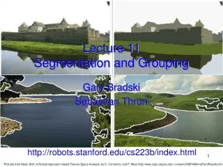
03/12/12 Grouping and Segmentation Computer Vision CS 543 / ECE 549 University of Illinois Derek Hoiem
Announcements • HW 3: due today • Graded by Tues after spring break • HW 4: out soon • Mean-shift segmentation • EM problem for dealing with bad annotators • Graph cuts segmentation
Today’s class • Segmentation and grouping • Gestalt cues • By clustering (mean-shift) • By boundaries (watershed)
Gestalt psychology or gestaltism German: Gestalt - "form" or "whole” Berlin School, early 20th century Kurt Koffka, Max Wertheimer, and Wolfgang Köhler • View of brain: • whole is more than the sum of its parts • holistic • parallel • analog • self-organizing tendencies Slide from S. Saverese
Gestaltism The Muller-Lyer illusion
Principles of perceptual organization From Steve Lehar: The Constructive Aspect of Visual Perception
Grouping by invisible completion From Steve Lehar: The Constructive Aspect of Visual Perception
Grouping involves global interpretation From Steve Lehar: The Constructive Aspect of Visual Perception
Grouping involves global interpretation From Steve Lehar: The Constructive Aspect of Visual Perception
Gestalt cues • Good intuition and basic principles for grouping • Basis for many ideas in segmentation and occlusion reasoning • Some (e.g., symmetry) are difficult to implement in practice
Image segmentation Goal: Group pixels into meaningful or perceptually similar regions
Segmentation for feature support 50x50 Patch 50x50 Patch
Segmentation for efficiency [Felzenszwalb and Huttenlocher 2004] [Shi and Malik 2001] [Hoiem et al. 2005, Mori 2005]
Segmentation as a result Rother et al. 2004
Types of segmentations Oversegmentation Undersegmentation Multiple Segmentations
Major processes for segmentation • Bottom-up: group tokens with similar features • Top-down: group tokens that likely belong to the same object [Levin and Weiss 2006]
Segmentation using clustering • Kmeans • Mean-shift
Feature Space Source: K. Grauman
K-means clustering using intensity alone and color alone Image Clusters on intensity Clusters on color
K-Means pros and cons • Pros • Simple and fast • Easy to implement • Cons • Need to choose K • Sensitive to outliers • Usage • Rarely used for pixel segmentation
Mean shift segmentation D. Comaniciu and P. Meer, Mean Shift: A Robust Approach toward Feature Space Analysis, PAMI 2002. • Versatile technique for clustering-based segmentation
Mean shift algorithm • Try to find modes of this non-parametric density
Kernel density estimation Kernel Estimated density Data (1-D)
Kernel density estimation Kernel density estimation function Gaussian kernel
Mean shift Region of interest Center of mass Mean Shift vector Slide by Y. Ukrainitz & B. Sarel
Mean shift Region of interest Center of mass Mean Shift vector Slide by Y. Ukrainitz & B. Sarel
Mean shift Region of interest Center of mass Mean Shift vector Slide by Y. Ukrainitz & B. Sarel
Mean shift Region of interest Center of mass Mean Shift vector Slide by Y. Ukrainitz & B. Sarel
Mean shift Region of interest Center of mass Mean Shift vector Slide by Y. Ukrainitz & B. Sarel
Mean shift Region of interest Center of mass Mean Shift vector Slide by Y. Ukrainitz & B. Sarel
Mean shift Region of interest Center of mass Slide by Y. Ukrainitz & B. Sarel
Computing the Mean Shift • Simple Mean Shift procedure: • Compute mean shift vector • Translate the Kernel window by m(x) Slide by Y. Ukrainitz & B. Sarel
Attraction basin • Attraction basin: the region for which all trajectories lead to the same mode • Cluster: all data points in the attraction basin of a mode Slide by Y. Ukrainitz & B. Sarel
Mean shift clustering • The mean shift algorithm seeks modes of the given set of points • Choose kernel and bandwidth • For each point: • Center a window on that point • Compute the mean of the data in the search window • Center the search window at the new mean location • Repeat (b,c) until convergence • Assign points that lead to nearby modes to the same cluster
Segmentation by Mean Shift • Compute features for each pixel (color, gradients, texture, etc); also store each pixel’s position • Set kernel size for features Kf and position Ks • Initialize windows at individual pixel locations • Perform mean shift for each window until convergence • Merge modes that are within width of Kf and Ks
Mean shift segmentation results http://www.caip.rutgers.edu/~comanici/MSPAMI/msPamiResults.html
http://www.caip.rutgers.edu/~comanici/MSPAMI/msPamiResults.htmlhttp://www.caip.rutgers.edu/~comanici/MSPAMI/msPamiResults.html
Mean-shift: other issues • Speedups • Binned estimation – replace points within some “bin” by point at center with mass • Fast search of neighbors – e.g., k-d tree or approximate NN • Update all windows in each iteration (faster convergence) • Other tricks • Use kNN to determine window sizes adaptively • Lots of theoretical support D. Comaniciu and P. Meer, Mean Shift: A Robust Approach toward Feature Space Analysis, PAMI 2002.
Doing mean-shift for HW 4 • Goal is to understand the basics of how mean-shift works • Just get something working that has the right behavior qualitatively • Don’t worry about speed • Simplifications • Work with very small images (120x80) • Use a uniform kernel (compute the mean of color, position within some neighborhood given by Kf and Ks) • Can use a heuristic for merging similar modes
Mean shift pros and cons • Pros • Good general-purpose segmentation • Flexible in number and shape of regions • Robust to outliers • Cons • Have to choose kernel size in advance • Not suitable for high-dimensional features • When to use it • Oversegmentation • Multiple segmentations • Tracking, clustering, filtering applications • D. Comaniciu, V. Ramesh, P. Meer: Real-Time Tracking of Non-Rigid Objects using Mean Shift, Best Paper Award, IEEE Conf. Computer Vision and Pattern Recognition (CVPR'00), Hilton Head Island, South Carolina, Vol. 2, 142-149, 2000
Watershed segmentation Watershed boundaries Image Gradient
Meyer’s watershed segmentation • Choose local minima as region seeds • Add neighbors to priority queue, sorted by value • Take top priority pixel from queue • If all labeled neighbors have same label, assign that label to pixel • Add all non-marked neighbors to queue • Repeat step 3 until finished (all remaining pixels in queue are on the boundary) Matlab: seg = watershed(bnd_im) Meyer 1991