Download
1 / 43
440 likes | 598 Views
Dynamic Phase Boundary Estimation using Electrical Impedance Tomography. By Umer Zeeshan Ijaz, Control Engineering Lab, Department of Electronic Engineering, Cheju National University, Cheju 690-756, Korea. (Supervised by Professor Kyung Youn Kim). Thesis Defense. Dated: 13.11.2007.

E N D
Dynamic Phase Boundary Estimation using Electrical Impedance Tomography By Umer Zeeshan Ijaz, Control Engineering Lab, Department of Electronic Engineering, Cheju National University, Cheju 690-756, Korea (Supervised by Professor Kyung Youn Kim) Thesis Defense Dated: 13.11.2007
CONTENTS • Introduction • Electrical Impedance Tomography • Boundary Representation • Fourier Coefficients • Front Points • Extended Kalman Filter • Kinematic Models • Interacting Multiple Model Scheme • Unscented Kalman Filter • Gauss-Newton Unscented Kalman Filter
INTRODUCTION Chemical engineers frequently encounter the flow of a mixture of two fluids in Liquid-gas or liquid-vapor mixtures condensers and evaporatorsgas-liquid reactors combustion systemstransport of some solid materials slurry of the solid particles in a liquid, and pumping the mixture through a pipe Liquid-liquid mixtures in emulsions as well as liquid-liquid extraction. Types of Flows
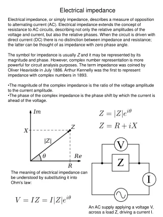
WHAT IS EIT? COMPUTER Reconstruction Algorithm Interface with Instrument I V Electrical Impedance Tomography(EIT) is a imaging modality in which the internal resistivity distribution is reconstructed based on the measured voltages on the surface object. Concept of electrical impedance tomography
FORWARD SOLVER VS INVERSE SOLVER Forward Solver Inverse Solver • The forward problem calculates the voltages on the electrodes by using the injected current and assumed resistivity distribution. • The inverse problem reconstructs the resistivity distribution by using the voltage measurements on the electrodes. An iterative inverse solver Forward vs. inverse problem for EIT
MATHEMATICAL MODEL: FORWARD SOLVER Governing Equation derived from Maxwell Equation Between electrodes, no current crosses the boundary if the impedance outside the imaged volume is much greater than that inside Boundary Conditions: Complete Electrode Model There is an existence of a thin, high-impedance layer beneath electrodes delivering current. This layer may be modelled as the limit of a thin layer of thickness d and impedance z/d as d goes to zero. (use ohm’s law) Beneath electrodes, neither potential nor the current crossing the boundary is known. Net current crossing the boundary beneath an electrode is equal to the current being delivered to it by tomograph electronics Constraints: For the solution to be unique
FEM DISCRETIZATION OF FORWARD PROBLEM L 3 4 N 2 1 1 N-Nodes, L-Electrodes, m-elementsP-Patterns 2 Potential inside: Potential on electrodes: Electrode area Basis function
CURRENT INJECTION PROTOCOL Opposite (L/2 Current Patterns) Current frame Adjacent (L Current Patterns) Trigonometric (L-1 Curent Patterns)
BOUNDARY INTERFACE REPRESENTATION 1/2 Truncated Fourier Coefficients Approach(Close Boundary)
BOUNDARY INTERFACE REPRESENTATION 2/2 σ=σ0 A0 C A1 σ=σ1 Front Points Approach (Open Boundary)
BOUNDARY INTERFACE FORWARD SOLVER 1/2 Forward Solver Inverse Solver Forward Solver Inverse Solver Changes required Boundary to Resistivity Profile Mapping (Forward Solver) Analytical Jacobians
BOUNDARY INTERFACE FORWARD SOLVER 2/2 Nj Al Sl Cl(s) σl s2 s1 Ar σr Sr Ni (b) (c) (e) (a) (d) (a) description of interface with front points /fourier coefficients b) mesh elements above the interface/inside the target are assigned one conductivity value ; (c) mesh elements below the interface/outside the target are assigned second conductivity value ; (d) mesh elements lying on the interface are assigned area average conductivity values assigned using equation ; and (e) final conductivity values at the end of assignment.
INVERSE SOLVER State Space Model Random-walk model Nonlinear measurement equation Linearizing the measurement equation about the predicted mean in the previous step Regularization
EXTENDED KALMAN FILTER (Front Points) Time Update Measurement Update Predefined Forward Solver Jacobian
EXTENDED KALMAN FILTER (Front Points) Results 10-Front Points, Contrast Ratio of 1:100, Moving every 4 Current Patterns (First two modes of cosine and sine with additional cosine in image reconstruction) 3% Noise Figure 2.14. Reconstructed images for scenario 2 with 3% white Gaussian noise. The solid line represents the true interface and the dotted line represents the estimated interface.
KINEMATIC MODEL (Fourier Coefficients) Bubble moving with constant velocity Bubble moving with constant acceleration Bubble expanding with constant acceleration Bubble expanding with constant velocity
OPTIMAL CURRENT PATTERN (Front Points) Distinguishability can be defined as a measurement ability to differentiate between homogeneous and inhomogeneous conductivities inside the domain. Power distinguishability is defined as the measured power change between the homogeneous and inhomogeneous cases, divided by the power applied in homogeneous case. 1 2 3 4 5 1. Trigonometric method with first 2 modes of cosine and sine (4 injections; 5 EKF states with repeated use of the first cosine)2. Opposite method with e1-e9 and e5-e13 pairs (2 injections; 5 states with repeated use of e1-e9, e5-e13, e1-e9)3. Cross method with e3-e7, e5-e13 pairs (2 injections; 5 states with repeated use of e3-e7, e5-e13, e3-e7)4. Opposite method with e3-e11, e7-e15 pairs (2 injections; 5 states with repeated use of e3-e11, e7-e15, e3-e11)5. Opposite method with e3-e11, e7-e15, e5-e13 pairs (3 injections; 5 states with repeated use of e3-e11, e7-e15). 1% Noise
KINEMATIC MODEL RESULTS (Fourier Coefficients) 6-Fourier Coefficients, Contrast Ratio of 1:106 , Moving every current Pattern Solid Line: Kinematic ModelDotted Line: Random-Walk Model Solid Line: True BoundaryDotted Line: Estimated Boundary a) Bubble moving with constant velocity b) Bubble expanding with constant velocity c) Bubble moving with constant acceleration d) Bubble expanding with constant acceleration
IMM SCHEME (Fourier Coefficients) 1/3 EKF1 EKF2 EKF3 T.U T.U T.U M.U M.U M.U *As error decreases, modelling probability increases
IMM SCHEME (Fourier Coefficients) 2/3 Mixing of estimates and error covariances Transition Probability EKF2 EKF3 EKF1 Predefined
IMM SCHEME (Fourier Coefficients) 3/3 Interacting/Mixing of the Estimates Linearization Filter 1 Filter M Model Probability Update State Estimation Combination EKF1 EKF2 EKF3 One-cycle flow diagram of the inverse solver with the IMM scheme.
IMM SCHEME RESULTS (Fourier Coefficients) 6-Fourier Coefficients, Contrast Ratio of 1:106, Moving after 8 current patterns EKF1 EKF2 EKF3 IMM
UNSCENTED TRANSFORM Actual (Sampling) Linearized (EKF) UT sigma points mean + + + + + + covariance + + + + + + + + + + + + + + + + + + + + + + + + + + + + + + + + + + + + + + + + + + + + + + + + + + + + + + + + + + + + + + + + + + + + + + + + + + + + + + + + + + + + + + + + + + + + + + + + + + + + + + + + + + + + + + + + + + + + + + + + + + + + + + + + + + + + + + + + + + + + + + + + + + + + + UT mean true mean + + + + + + + + + + + + + + + + + + + + + + + + + + + + + + + + + + + + + + + + + + + + + + + + + + + + + + + + + + + + + + + + + + + + + + + + + + + + + + + + + + + + + + + + + + UT covariance EKF mean transformed sigma points EKF covariance (a) (b) (c) An example of unscented transform for mean and covariance propagation: a) actual; (b) first-order linearization (EKF); and (c) unscented transform
UNSCENTED KALMAN FILTER (1/4) Run the state equation Generate 2n+1 sigma points where n is the size of augmented vector Calculate predicted mean and covariance Each point is the augmented vector State Space Model:
UNSCENTED KALMAN FILTER (2/4) Run the measurement equation and find the mean Create covariance matrices The sigma points should move towards the mean and at the same time, the sigma points on x domain should move towards the mean Time update complete
UNSCENTED KALMAN FILTER (3/4) Usually 2 for Gaussian distribution Calculate the gain and update the estimates and error covariance matrices Define weights Actual measurement True value where Usually zero Spread of sigma points, usually1e-3 Composite scaling parameter Measurement update complete
UNSCENTED KALMAN FILTER (4/4) Nonlinear Measurement Equation [FEM Forward Solver] k - + State Equation Weighted Mean Weighted Covariance Kalman Gain k=k+1 Block diagram of unscented Kalman filter for phase boundary estimation
UKF RESULTS (Fourier Coefficients) 32 Electrodes, 6-Fourier Coefficients, Contrast Ratio of 1:106, Moving after 6 current patterns Phantom solid line : true, dotted line : EKF, dashed line : UKF Plastic Target
UKF RESULTS (Front Points) 10-Front Points, Contrast Ratio of 1:100, moving every current pattern 2% Noise Rippled surface 3% Noise <EKF: -x- UKF : -o- >
GAUSS-NEWTON UNSCENTED KALMAN FILTER State Space Model Online State Equation Offline Gauss-Newton Measurement Update
GNUKF RESULTS (Front Points) 1% Noise 2% Noise 3% Noise
RESEARCH MILESTONES Front points (open boundary) Fourier coefficients (close boundary) -Analytical Jacobian used -successful till 16 Frontpoints -Contrast ratio of 1:10000 -3% Relative Noise -Current patterns reduced to 4 / target remains static with 16 electrodes configuration based on distinguishability analysis for EKF -Extended Kalman Filter and Unscented Kalman filter (recent) formulation for online monitoring -Gauss Newton Unscented Kalman filter formulation for improvement over unscented Kalman filter -With Unscented Kalman Filter and Gauss Newton Unscented Kalman Filter, image reconstruction using 1 current pattern is also possible. -Analytical Jacobian used -6 coefficients to represent an elliptic object, can go for more, however, higher coefficients are quite sensitive -Contrast ratio of 1:1000000 -3% Relative Noise -Current patterns reduced to 6 / target remains static in experiments with 32 electrodes configuration. -Extended Kalman Filter and Unscented Kalman filter (recent) formulation for online monitoring -Interacting Multiple Model Scheme for time-varying process noises -Kinematic models (velocity, acceleration) done for movement of air bubbles, void fractions
APPENDIX: Derivation of Jacobian 1/10 In some cases, the voltages are measured only at some selected electrodes, not every electrode. Also, the selected electrodes may be different at each current pattern. The measured voltages at the measurement electrodes can be obtained as where, is the number of the measurement electrodes and is the measurement matrix. The element is set to ‘1’ if the -th electrode is measured at the -th current pattern and otherwise set to zero. Furthermore, can be extracted directly from by introducing the extended mapping matrix and where . Therefore, we have where the extended measurement matrix is defined as If the pseudo-resistance matrix defined as or is given we can calculate the Jacobian matrix. The pseudo-resistance matrix can be easily obtained during the solution of the system equation or and where
APPENDIX: Derivation of Jacobian 2/10 Front Points Approach Jacobian:
APPENDIX: Derivation of Jacobian 3/10 Since we are considering the stratified flow of two immiscible liquids therefore, the matrix B will be
APPENDIX: Derivation of Jacobian 4/10 Assuming that the interface is represented by a set of linear piecewise interpolation functions: , unit pulse defined for Any small perturbation of results in small perturbation in and in where
APPENDIX: Derivation of Jacobian 5/10 Considering the interface for mesh crossing elements where For a small perturbation inonly and will change The function can be expanded about the interface Finally, we have
APPENDIX: Derivation of Jacobian 6/10 Five types of interface-crossing elements in case of an arbitrarily small perturbation of in There are five types of interface-crossing elements when is perturbed by an arbitrarily small perturbation of . Assume that there are only two intersections of the interface and the mesh faces and the intersections are denoted as is constant in a certain mesh, and where . Recalling that the integration for each type will be evaluated as . TYPE 1: TYPE 2: TYPE 3: TYPE 4: TYPE 5:
APPENDIX: Derivation of Jacobian 7/10 Fourier Coefficients Approach The derivative of the stiffness matrix with respect to the coefficient is
APPENDIX: Derivation of Jacobian 8/10 In order to obtain the Jacobian, now, let us consider the evaluation of the expression We define a new coordinate system where is the positively oriented coordinate along the closes curve , and is the coordinate outward normal from the region The perturbed boundary will be Therefore,
APPENDIX: Derivation of Jacobian 9/10 The Jacobian for the transformation of the coordinate will be The function can be expanded about the boundary We have
APPENDIX: Derivation of Jacobian 10/10 In this, is evaluated at the boundary . When differentiating with respect to , that is perturbing , we have and .On the other hand when differentiating with respect to , we have and . Finally, the derivative of the matrix with respect to the coefficients becomes where denotes the set of elements crossing If , and constant in each element, we have