Download
1 / 14
140 likes | 144 Views
Supernova Extinctions and Unfolding Matrix. Johanna-Laina Fischer With Professor David Cinabro of Wayne State University. Supernova: A Definition. Exploding star Can become billions of times as bright as the sun Gradually fades from view At max brightness, may outshine an entire galaxy

E N D
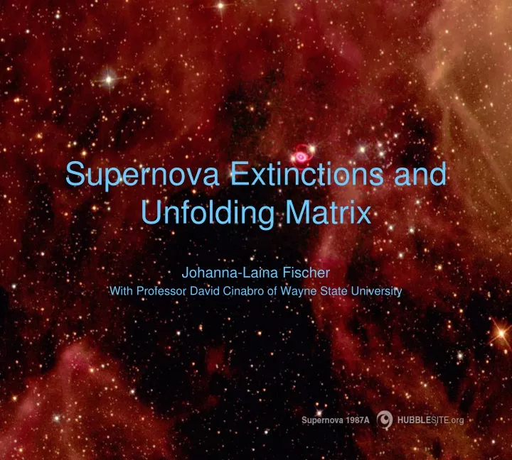
Supernova Extinctions and Unfolding Matrix Johanna-Laina Fischer With Professor David Cinabro of Wayne State University
Supernova: A Definition • Exploding star • Can become billions of times as bright as the sun • Gradually fades from view • At max brightness, may outshine an entire galaxy • Throws a large cloud of dust and gas into space X-ray, Optical & Infrared Composite of Kepler's Supernova Remnant
Abstract/Background • Problem • Light extincted by dust and gas • Milky Way Galaxy and Host Galaxy • Redshift and extinction cause dimming and reddening • Dimmed light measured a function of wavelength • At short wavelengths we have reddening, which is not the same as redshift • Need accurate measure of apparent brightness • The Challenge/Goal • Disentangle the effects of redshift and extinction for poorly measured redshifts • Why are they badly measure? • Distance • Technology not up to par • Extinction parameterized by the variable Av
Abstract/Background (Cont’d) • Focus/Goal of Project • Find method for obtaining best measure of Av • Use simulated 1A supernova light curves • Fit known light curve models • Identifying catastrophic failures (Av) • Eliminating failures • Results have excellent measure of extinction • Not efficient • Method will be applied to a set of real 1a’s from the Sloan Digital Sky Survey • Unfolding Matrix • If Goal Reached • More supernova available for use • More information gathered about our Universe • History • Fate
Research Plan/Procedure: Supernova Extinctions • Preferred way to measure extinction would be spectroscopy • Spectroscopy: precisely measures light output vs. wavelength • Supernova too far away • Not enough light available to make a spectrum • Second choice is photometry • Photometry: light curves observed in broad range of wavelengths using filters • Filters denoted U, G, R, I, and Z in SDSS • The differences of the fluxes in broad wavelength filters are called ‘colors’ • Fit light curve simultaneously for redshift and extinction by assuming an underlying model of supernova light curve • Redshift and Extinction are highly correlated • Correlation gets stronger as redshift gets larger, light curve not measured as well • Supernova farther away at larger redshifts • Hard to tell if supernova is dim or red • At greater distances, more extinction (dust and gas)
Research Plan/Procedure (Cont’d) • Fits that give a large uncertainty of the photometric redshift, fit a second time • Constraint on redshift to match the redshift of its host galaxy • Large fraction of supernova light curves have badly measured extinction. • Want these eliminated • Look at specific aspects of light curves simulated by SNANA light curve simulator • Difference between Photometrically Measured Redshift and Simulated Redshift • Difference between Average Extinction and Simulated Average Extinction • Simulated Average Extinction • Number of Degrees of Freedom in the fit to the light curve • Errors between the Host Galaxy’s Redshift and Photometrically Measured Redshift • Errors of the Host Galaxy’s Redshift • Errors of the Photometrically measured redshift
Data/Graphs:Simulation Av-SimAv The graph without had great tailing, slight right tailing. Estimated Domain: -1.0 to 1.3 The graph with all of the cuts had a slight left tailing but a well improved graph. Estimated Domain: -0.7 to 0.6
Procedure: Unfolding Matrix • Unfolding Matrix gives us an idea of what the data's values of average extinction actually are • When applied to the data, we find the underlying average extinction distribution • which is what the average extinction truly looks like • Unravel the unfolding matrix • Run a large simulation • Set to have simulated data values that were not constrained to the host galaxies' redshift • Data fit to a light curve • Used predetermined cuts to deem “good” from “bad” data • Made graphs for average extinction of simulated data (Av) and, as well as the simulated average extinction (SimAv) • Simulated average extinction graph was cut into bins • Summed and normalized the average extinction based on bins • Graphs added together and underlying average extinction distribution is found
Unfolding Matrix and Average Extinction Comparison In the simulated data, the unfolding matrix agrees with the average extinction graph that was generated. In both the unfolded and generated graphs, we find that the means are fairly small as are the RMS values. When comparing the unfolded and generated graphs in the simulation, the means and RMS values have a difference between the two at about 0.03. Again, both of the mean and RMS values are fairly small.
Unfolding Matrix Fit to Exponential Curve When the unfolding matrix is fit to an exponential curve, the result gives us a χ2 value of 0.818.
Conclusion • In the simulated data, many cuts needed to be made. • We determined “Bad” supernova (catastrophic failures) and cut them out • “Bad”: Photoz and Av measurements better or worse than the reading. • More accurate comparison of data when eliminated • Other cuts made, cuts ensure precise and small RMS and accurate means consistent with zero • Cuts can be manipulated onto real Type 1A supernovae • Problem: SimAv is not in real data • Cannot be used, but used to monitor fits in simulated data • Findings • If the redshift is not measured well, extinction is not measured well, intrinsic brightness wrong • When intrinsic brightness is wrong, cosmology wrong • By cosmology we can start to understand the explosive origin of our universe as well as its sad fate • As seen in the previous graph, it is most important that the unfolding matrix graph agrees with the graph that was generated
Bibliography • M. Bolzonella et al. (2000). "Photometric z based on standard SED fitting procedures". Astronomy and Astrophysics. Retrieved from: http://arxiv.org/PS_cache/astro-ph/pdf/0003/0003380v2.pdf. • Wang, Y. (2008). "A Model-Independent Photometric Redshift Estimator Type IA Supernovae". Astronomy and Astrophysics. Retrieved from: http://arxiv.org/PS_cache/astro-ph/pdf/0609/0609639v2.pdf. • Comins, N.F., Kaufmann III, W.J. (2000). "Discovering the Universe 5.0". New York. W.H. Freeman and Company. Pages 99, 262, 310-311, 399. • Cummings, K., Laws, P.W., et al. (2004?). “Understanding Physics”. John Wiley & Sons. • The Hubble Heritage Team. (1987, 1994, 1996-1997). “SN1987A in the Large Magellanic Cloud”. Retrieved from: http://hubblesite.org/newscenter/archive/releases/1999/04/image/a/ • Professor David Cinabro • Brecher, Kenneth. "Supernova." World Book Online Reference Center. 2005. World Book, Inc. http://www.worldbookonline.com/wb/Article?id=ar540310.