Download
1 / 58
580 likes | 927 Views
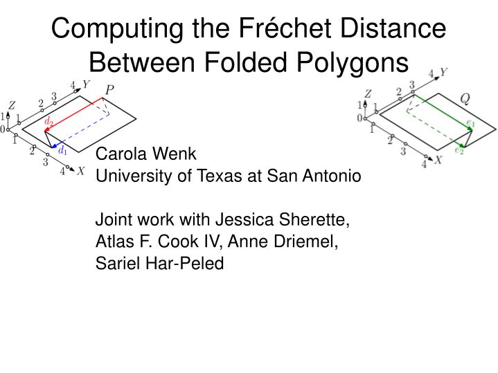
Computing the Fr é chet Distance Between Folded Polygons. Carola Wenk University of Texas at San Antonio Joint work with Jessica Sherette, Atlas F. Cook IV, Anne Driemel, Sariel Har-Peled. Outline. Preliminaries Simple Polygons Algorithm Folded Polgons Diagonal Monotonicity Test

E N D
Computing the Fréchet Distance Between Folded Polygons Carola WenkUniversity of Texas at San Antonio Joint work with Jessica Sherette, Atlas F. Cook IV, Anne Driemel, Sariel Har-Peled
Outline • Preliminaries • Simple Polygons Algorithm • Folded Polgons • Diagonal Monotonicity Test • Untangling Image Curves • Folded Polygons Algorithms • Fixed Parameter Tractable Algorithm • Approximation Algorithm • Special Variants of Folded Polgons • Conclusion
Fréchet Distance for Curves • Dog walking example • Person is walking a dog (person on one curve, dog on the other) • Allowed to control their speeds but not allowed to go backwards • Fréchet distance of the curves: minimal leash length necessary for both to walk the curves from beginning to end A B
Fréchet Distance for Surfaces s: [0,1]2 [0,1]2 p [0,1]2 where ranges over orientation preserving homeomorphisms. • Usually: Piecewise linear surfaces in R3. • Let A,B: [0,1]2Rd be two surfaces • dF(A,B) = inf max ||A(p) – B(s(p))||
Fréchet Distance between Surfaces • Computing the Fréchet distance between surfaces is NP-hard • One triangle, one triangulated surface [G98] • Two polygons with holes or two terrains [BBS10] • The Fréchet distance between surfaces is upper semi-computable [AB10]. It is not known whether it is computable. • The Fréchet distance between two simple polygons can be computed in polynomial time [BBW08] • We extend this algorithm to “folded” polygons
Simple Polygons Algorithm [BBW08] • It is easy to compute the Fréchet distance between closed polygonal curves • The Fréchet distance between a convex polygon and a simple polygon is the same is that between their boundary curves. • Idea: Restrict the class of mappings to consider • Given two simple polygons P and Q • Divide them up into matched pairs of convex polygons and simple polygons. • Then use the approach above to check whether the distance is within some .
Simple Polygons Algorithm • “diagonals” in P are the line segments in a convex subdivision of P • “edges” in Q are the line segments in a convex subdivision of Q • [BBW08] demonstrate that it suffices to consider mappings that map • ∂P onto ∂Q such that dF(∂P,∂Q) e • diagonals in P to shortest paths in Q with Fréchet distance e
Simple Polygons Algorithm • “diagonals” in P are the line segments in a convex subdivision of P • “edges” in Q are the line segments in a convex subdivision of Q • [BBW08] demonstrate that it suffices to consider mappings that map • ∂P onto ∂Q such that dF(∂P,∂Q) e • diagonals in P to shortest paths in Q with Fréchet distance e
Folded Polygons • We extend this algorithm to non-flat surfaces. • Specifically, we consider piecewise linear surfaces with a convex subdivision which has an acyclic dual graph (“folded polygons”)
Shortest Paths? • The simple polygons algorithm maps diagonals in one surface to shortest paths in the other surface. • For folded polygons, mapping a diagonal onto a shortest path is not necessarily optimal.
Shortest Path Counter Example • s1 is the shortest path between a and b,but the diagonal d has smaller Fréchet distance to s2 than to s1.
Fréchet Shortest Paths • Fréchet shortest paths = paths with Fréchet distance eto a given diagonal • The shortest path between two points on the boundary of Q crosses some sequence of edges. • We prove that any Fréchet shortest path between those points crosses the exact same edge sequence. Q
Fréchet Shortest Paths • Like the shortest path, we can prove that the portion of a Fréchet shortest path between two adjacent edges in Q consists of a line segment.
Diagonal Monotonicity Test • Greedy O(n) algorithm to decide if there exists a path between two points on Q within Fréchet distance e of a diagonal. (n = # edges in Q). • P and Q “pass the diagonal monotonicity test for e” iff • dF(∂P,∂Q) e (this specifies a mapping of the diagonal endpoints) • For every diagonal in P, a Fréchet shortest path with distance at most e to the diagonal exists.
Problem of Tangled Image Curves • The image curves may cross (“tangle”) • In this case, the subdivision of Q is no longer valid. • We need to ensure that these image curves can be untangled.
Problem of Tangled Image Curves • Unfortunately, there exist cases were these image curves are forced to tangle. • In the example pictured below P and Q pass the diagonal monotonicity test for e = 1 (i.e., dF(∂P,∂Q) 1, and there exist Fréchet shortest paths with Fréchet distance 1 to the diagonals).
Problem of Tangled Image Curves • But the image curves for d1 and d2must cross out of order along the edges e1 and e2 for e =1. Thus we do not have a homeomorphism between P and Q. • Therefore, even if P and Q pass the diagonal monotonicity test for e, the Fréchet distance between P and Q may be greater than e.
Results To ensure a homeomorphism exists between the surfaces we must address such tangles. We consider three approaches: • Compute the constraints posed by such tangles directly. fixed parameter tractable algorithm • Use an approximation algorithm which avoids the tangles altogether. poly-time approx. algorithm • Consider a special non-trivial class of folded polygons for which we can use shortest paths instead of Fréchet shortest paths. poly-time algorithm
1) Computing Tangle Constraints Directly • Fixed parameter tractable algorithm, assumes constant number of edges and diagonals. • A point is in the “untanglea-bility space” for an edge e iff the image curves can be untangled on e for the specified points.
2) Approximation Algorithm • Suppose P and Q pass the diagonal monotonicity test for e. We prove that dF(P,Q) 9e . • We can then optimize this e in polynomial time using binary search and the diagonal monotonicity test. Thus, we have a 9-approximation algorithm. Plug the diagonal monotonicity test into the polynomial-time simple polygons algorithm • So, how do we prove dF(P,Q) 9e ?
9-Approximation: Proof Sketch • Choose a diagonal d in P which cuts off an ear. • To have a homeomorph-ism between P and Q the image curve of d in Q, call it d', must also cut off an ear. • If another image curve d’1 crosses d‘ then we no longer have a homeomorphism.
9-Approximation: Proof Sketch • Idea: Let's map d to the “upper envelope” of the image curves, call it d’’. • How much do we need to increase e to do this?
9-Approximation: Proof Sketch • Consider the pre-images of the points where d' and d'1cross. • We can use these to bound how far d is from the part of d'1 that crosses above it.
9-Approximation: Proof Sketch • Consider mapping from a to a' and then to a1. Likewise from b to b' to b1. • From this follows that dF(ab,a1b1) 2e .
9-Approximation: Proof Sketch • Thus for each point on ab we can first map it to a point on a1b1 within distance 2*e and then map it to a point on d’1 within distance e. • Therefore, ab can be mapped to the part of d’1 between a' and b' within distance 3* e .
9-Approximation: Proof Sketch • If d’1 then crosses another image curve d’2 this poses a problem. • Their crossing will have two pre-images on d. One from using the previous reasoning on d1. Another from using it on d2.
9-Approximation: Proof Sketch • Nonetheless each pre-image on d of the crossing cannot be more than 3e away from it. • Thus they cannot be separated along d by more than 6e. • We can approximate all these intersections away with a total of 9e.
9-Approximation: Proof Sketch • We must also show that if these 6e-regions occur out of order on d we can approximate them away as well. • Can be proven through technical case analysis. • In the end, incrementally cut off ears from P and map to Q, in order to obtain an overall mapping witnessing dF(P,Q) 9e .
3) Special Variants of Folded Polygons • We show that in the following special variants of folded polygons, using L∞, we can map diagonals to shortest paths rather than Fréchet shortest paths. • Perpendicular: All diagonals of P are parallel to one axis, and all edges of Q are perpendicular to this axis (and parallel to one of the other axes) • Parallel: All diagonals of P and Q are parallel to one axis. • Mixed: All diagonals of P and Q are parallel to the x-axis, y-axis, or z-axis. Use the polynomial-time simple polygons algorithm
Half-Space Lemma • Let R be a half space with boundary parallel to the xy-, xz-, or yz-plane. • Let Q be a folded polygon with edges parallel to one axis • If a (Fréchet shortest) path between two points is completely contained in R so is the shortest path. Q
Half-Space Lemma • The proof of the lemma involves checking a few cases to show that no positioning of the edges can “force” the shortest path to go outside of R.
Perpendicular Variant • Let P be a folded polygon with all of its diagonals parallel to one axis. • Let Q be a folded polygon with all of its edges perpendicular to this axis, and parallel to one of the other axes. • For a given diagonal d in P and a Fréchet shortest path, consider any edgee in Q that is crossed by the image curve of d. d e
Perpendicular Variant • Take a point on d. Either: • It is within e distance to no points on e. • It is within e distance to some fixed set of points on e. • (2D pictures but similar in 3D) d d e e
Perpendicular Variant • We can prove that the shortest path will always cross in the reachable regions on each of the edges using the half-space lemma.
Perpendicular Variant: Proof Sketch • The idea is we use these half spaces to represent constraints on the diagonal d that can be mapped to. • In the picture the intersection of the half spaces contains exactly those points within e distance of some point on the diagonal d. (using L∞; similar in 3D)
Perpendicular Variant: Proof Sketch • Since we know some path between these points exists which is completely inside the intersection, we also know that the shortest path between the points is completely inside the intersection.
Perpendicular Variant • We can then change the pre-image point of each crossing for an edge so that it maps to the crossing for the shortest path.
Perpendicular Variant • We can then change the pre-image point of each crossing for an edge so that it maps to the crossing for the shortest path. • Thus, if a diagonal is within Fréchet distance e of any path between two points, then it is also within Fréchet distance e of the shortest path.
Parallel Variant • Let P and Q be two folded polygons with all of their diagonals and edges parallel to an axis. • For a given diagonal d in P and a Fréchet shortest path, consider any edgee in Q that is crossed by the image curve of d.
Parallel Variant: Proof Sketch • Again, by using the half-space lemma we can then show that if some path crosses each edge at a point within distance e of some point on d, so does the shortest path. • (Where d is the diagonal we want to map to the shortest path).
Parallel Variant: Proof Sketch • Unlike in the perpendicular case, when using the shortest path, the pre-images of the resulting crossing points on the diagonal may occur out of order. • If this happens we would no longer have a monotone mapping between the diagonal and the shortest path.
Parallel Variant: Proof Sketch • This is similar to the problem we had in the approximation algorithm proof. • Unlike before, when we approximated them away, we can actually show that these points can be chosen in order along the diagonal.
Parallel Variant: Proof Sketch • This problem arises when the shortest path zigzags back and forth. • Using two applications of our lemma we can show that for any pair of edges this zigzag will be no worse for the shortest path than it is for any other path between the same points.
Parallel Variant: Proof Sketch • We first choose a point b which lies on the shortest path between a and c and between the problem edges. • We can then show the shortest path can't go too far to the right on e1.