Download
1 / 26
260 likes | 264 Views
This course covers the historical background, principles and applications of Statistical Parametric Mapping (SPM) in functional magnetic resonance imaging (fMRI), positron emission tomography (PET), and voxel-based morphometry (VBM).

E N D
Statistical Parametric Mapping for fMRI, PET and VBM Ged Ridgway Wellcome Trust Centre for Neuroimaging UCL Institute of Neurology SPM Course October 2011
Contents • Historical background • Positron emission tomography (PET) • Statistical parametric mapping (SPM) • Functional magnetic resonance imaging (fMRI) • Voxel-based morphometry
Part I: 19th Century (!) • Angelo Mosso, Turin 1846 – 1910 Figures fromDavid Heeger
Part I: 19th Century (!) • Early evidence for functional segregation from damage • E.g. Phineas Gage, 1823-1860, studied by John Martyn Harlow, 1819-1907.“Previous to his injury he possessed a well-balanced mind … the equilibrium between his intellectual faculties and animal propensities, seems to have been destroyed. He is fitful, irreverent, indulging in the grossest profanity” From the collection of Jack and Beverly Wilgus
Haemodynamics • Roy & Sherrington (1890), On the Regulation of the Blood-supply of the Brain, J Physiol 11(1-2) • Fulton (1928)Observations upon the vascularity of the human occipital lobe during visual activity, Brain 51(3) • Raichle (1998), PNAS 95(3):765-772 • “introduction of an in vivo tissue autoradiographic measurement of regional blood flow in laboratory animals by Kety’s group provided the first glimpse of quantitative changes in blood flow in the brain related directly to brain function” • William Landau [in Kety’s group]: “this is a very secondhand way of determining physiological activity; it is rather like trying to measure what a factory does by measuring the intake of water and the output of sewage. This is only a problem of plumbing”
Haemodynamics • Please see Kerstin Preuschoff’s Zurich SPM Course slides for more Friston et al. (2000) NeuroImage 12:466-477
Positron emission tomography (PET) • A tracer (radionuclide) emits a positron, which annihilates with an electron, emitting a pair of gamma rays in opposite directions • The detected lines can be grouped into projection images (sinograms) and reconstructed into tomographic images • Different tracers allow various properties to be measured • 15O can measure blood flow relatively quickly (<1 min) but requires a cyclotron because of its short 2 minute half-life • 18F Fluorodeoxyglucose (FDG) measures glucose metabolism, and has a half life of 110 minutes • Other tracers exist that bind to interesting receptors (e.g. dopamine, serotonin) or beta-amyloid plaques
Parametric mapping • Early PET focussed on quantitation of parameters • See also Lammertsma & Hume (1996) [source of figure] • Prof Terry Jones interviewed by UCL Centre for History of Medicine:“It was as if I could take a bit of my brain out and then put it into a laboratory well counter … how many megabecques or microcuries of radioactivity per ml of tissue … I pointed out if we could measure the concentration in the artery and the tissue at the same time, you could solve these equations for blood flow and oxygen consumption”
Statisticalparametric mapping • Often the interest is not the quantities, but their differences in different conditions • Terry Jones: “And here was this guy Friston, sort of running roughshod over all this [quantitation], and saying, ‘Oh, I’ll take five of those, and five of those, and look for statistical differences…”
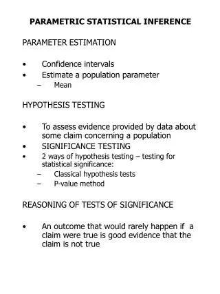
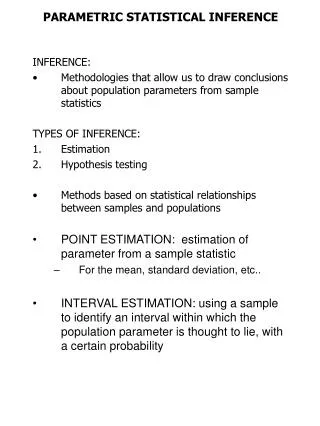
Statistical parametric mapping • Some questions you might ask at this point • Can we test more interesting hypotheses than condition A vs. B? • Answer: The general linear model and experimental design • How significant is a particular voxel’s t-score, given consideration of so many voxels over the brain? • Multiple comparison correction using random field theory • What if the subject moves during the scan or between scans? How can we report locations of findings? How can we combine data from multiple subjects? • Image registration and spatial normalisation; hierarchical models • What about functional integration of multiple brain regions? • Functional and effective connectivity, dynamic causal modelling
Image time-series Statistical Parametric Map Design matrix Spatial filter Realignment Smoothing General Linear Model StatisticalInference RFT Normalisation p <0.05 Anatomicalreference Parameter estimates
Functional magnetic resonance imaging (fMRI) • Some disadvantages of PET • Slow, even compared to haemodynamic delays • Low spatial resolution • Ionising radiation • Magnetic resonance imaging • Quantum mechanical property of spin, e.g. of hydrogen nuclei • Spins align with and precess around an applied magnetic field • Inputting RF energy perturbs the established equilibrium and puts spins in phase with each other; a signal can be measured • Spins relax back to equilibrium and de-phase with each other • Different longitudinal (T1) and transverse (T2) relaxation times • Field inhomogeneities accelerate the T2 relaxation (T2*)
Functional magnetic resonance imaging (fMRI) • Blood contains oxygenated and deoxygenated haemoglobin, with different magnetic properties • Paramagnetic deoxyhaemoglobin distorts the magnetic field, leading to faster T2* decay • The influx of blood following activity changes the proportion of oxy- and deoxyhaemoglobin, and hence the T2 or T2*-weighted MRI signal • This Blood Oxygenation Level Dependent (BOLD) effect allows functional imaging with MRI See also Kerstin’s slides and Ogawa & Sung (2007)
More Karl on the BOLD effect • Friston (2009) • How many times have you read, “We know very little about the relationship between fMRI signals and their underlying neuronal causes”? • In fact, decades of careful studies have clarified an enormous amount about the mapping between neuronal activity and hemodynamics • Furthermore, we know more than is sufficient to use fMRI for brain mapping. This is because the statistical modelsused to infer regionally specific responses make no assumptions about how neuronal responses are converted into measured signals
The imaging bit of MRI… • … is complicated! • The rate of precesssion is field-strength dependent • Electromagnetic coils can setup spatial gradients in field-strength, which cause gradients in precession frequency • A frequency gradient persisting for a certain time establishes a sinusoidal phase gradient • The overall signal is stronger if the spatial frequency of the object (e.g. some cortical folds) matches this • Can effectively measure the 2D Fourier transform or spectrum of an object, and hence reconstruct an image
The imaging bit of MRI… • MRI from picture to proton has one of the clearest explanations and some great examples of how spatial frequency space (k-space) relates to features in the image space
Temporal modelling of fMRI data • With PET we can acquiring some scans in one condition and some in another, and test statistically for differences • With fMRI, we typically acquire a scan every few seconds, and wish to study “event-related” responses • (also recently sub-second sampling, e.g. Feinberg et al., 2009) • We do this by creating a model of what the haemodynamic response to a sequence of events or conditions would look like in time (with its ~6s delay, undershoot, etc.) and fitting this model to the data
Model specification Parameter estimation Hypothesis Statistic Voxel-wise time series analysis Time Time BOLD signal single voxel time series SPM
Multiple subjects and standard space The TalairachAtlas (single subject, post-mortem) The MNI/ICBM AVG152 Template(average of 152 in-vivo MRI)
Computational anatomy • If we can estimate the transformations that align and warp each subject to match a template, then we can study individual differences in these transformations or derivatives • E.g. deformation-based and tensor-based morphometry • Changes in local volume are interesting and interpretable
Voxel based morphometry (VBM) • VBM involves creating spatially normalised images, whose intensities at each point relate to the local volume of a particular brain tissue (e.g. gray matter) at the corresponding point in the original (unnormalised) image • This requires tissue segmentation, spatial normalisation, and a “change of variables” to account for volume changes occuring in the normalisation process • Spatial smoothing helps to ameliorate residual anatomical differences after imperfect normalisation • The same general linear modelling & RFT machinery in SPM can then be used to study differences in structure
Image time-series Statistical Parametric Map Design matrix Spatial filter Realignment Smoothing General Linear Model StatisticalInference RFT Normalisation p <0.05 Anatomicalreference Parameter estimates
SPM Documentation SPM Books:Human Brain Function I & II Statistical Parametric Mapping Peer reviewed literature Online help & function descriptions SPM Manual