Download
1 / 26
290 likes | 776 Views
The general linear model and Statistical Parametric Mapping II: GLM for fMRI. Alexa Morcom and Stefan Kiebel, Rik Henson, Andrew Holmes & J-B Poline. Overview. Introduction General linear model(s) for fMRI Time series Haemodynamic response Low frequency noise

E N D
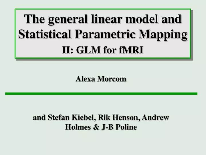
The general linear model and Statistical Parametric MappingII: GLM for fMRI Alexa Morcom and Stefan Kiebel, Rik Henson, Andrew Holmes & J-B Poline
Overview • Introduction • General linear model(s) for fMRI • Time series • Haemodynamic response • Low frequency noise • Two GLMs fitted in 2-stage procedure • Summary
Modelling with SPM Design matrix Contrasts Preprocessed data: single voxel Parameter estimates General linear model SPMs
GLM review • Design matrix – the model • Effects of interest • Confounds (aka effects of no interest) • Residuals (error measures of the whole model) • Estimate effects and error for data • Specific effects are quantified as contrasts of parameter estimates (aka betas) • Statistic • Compare estimated effects – the contrasts – with appropriate error measures • Are the effects surprisingly large?
fMRI analysis • Data can be filtered to remove low-frequency (1/f) noise • Effects of interest are convolved with haemodynamic (BOLD) response function (HRF), to capture sluggish nature of response • Scans must be treated as a timeseries, not as independent observations • i.e. typically temporally autocorrelated (for TRs<8s)
fMRI analysis • Data can be filtered to remove low-frequency (1/f) noise • Effects of interest are convolved with haemodynamic (BOLD) response function (HRF), to capture sluggish nature of response • Scans must be treated as a timeseries, not as independent observations • i.e. typically temporally autocorrelated (for TRs<8s)
aliasing power spectrum noise Low frequency noise • Physical (scanner drifts) • Physiological (aliased) • cardiac (~1 Hz) • respiratory (~0.25 Hz) • Low frequency noise: • Physical (scanner drifts) • Physiological (aliased) • cardiac (~1 Hz) • respiratory (~0.25 Hz) power spectrum highpass filter signal (eg infinite 30s on-off)
fMRI example One session Time series of BOLD responses in one voxel Passive word listening versus rest 7 cycles of rest and listening Each epoch 6 scans with 7 sec TR Stimulus function Question: Is there a change in the BOLD response between listening and rest?
Regression model Single subject No. of effects in model + + = Number of scans No. of effects in model Number of scans * 1 1 1
Add high pass filter Single subject This means ‘taking out’ fluctuations below the specified frequency SPM implements by fitting low frequency fluctuations as effects of no interest
Raw fMRI timeseries Fitted & adjusted data
Raw fMRI timeseries Fitted & adjusted data highpass filtered (and scaled) fitted high-pass filter
Raw fMRI timeseries Fitted & adjusted data Adjusted data fitted box-car highpass filtered (and scaled) fitted high-pass filter
Raw fMRI timeseries Fitted & adjusted data Adjusted data fitted box-car highpass filtered (and scaled) Residuals fitted high-pass filter
Regression model Single subject + + = (High-pass filter not visible) * 1 1 1
Regression model Single subject = + + * 1 1 1 • Stimulus function is not expected BOLD response • Data is serially correlated What‘s wrong with this model?
fMRI analysis • Data can be filtered to remove low-frequency (1/f) noise • Effects of interest are convolved with haemodynamic (BOLD) response function (HRF), to capture sluggish nature of response • Scans must be treated as a timeseries, not as independent observations • i.e. typically temporally autocorrelated (for TRs<8s)
Unconvolved fit Residuals hæmodynamic response Convolution with HRF = Boxcar function convolved with HRF
Unconvolved fit Residuals hæmodynamic response Convolved fit Convolution with HRF = Boxcar function convolved with HRF Residuals (less structure)
fMRI analysis • Data can be filtered to remove low-frequency (1/f) noise • Effects of interest are convolved with haemodynamic (BOLD) response function (HRF), to capture sluggish nature of response • Scans must be treated as a timeseries, not as independent observations • i.e. typically temporally autocorrelated (for TRs<8s
Temporal autocorrelation • Because scans are not independent measures, the number of degrees of freedom is less than the number of scans • This means that under the null hypothesis the data are less free to vary than might be assumed • A given statistic, e.g. T value, is therefore less surprising and so less significant than we think… • …the next talk
2-stage GLM ‘Summary statistic’ random effects method Each has an independently acquired set of data These are modelled separately Models account for within subjectsvariability Parameter estimates apply to individual subjects 1st level Single subject Single subject contrasts of parameter estimates taken forward to 2nd level as (spm_con*.img) ‘con images‘
2-stage GLM ‘Summary statistic’ random effects method Each has an independently acquired set of data These are modelled separately Models account for within subjectsvariability Parameter estimates apply to individual subjects 1st level Single subject Single subject contrasts of parameter estimates taken forward to 2nd level as (spm_con*.img) ‘con images‘ To make an inference that generalises to the population, must also model the between subjects variability 1st level betas measure each subject’s effects 2nd level betas measure group effect/s Group/s of subjects 2nd level Statistics compare contrasts of 2nd level parameter estimates to 2nd level error
Single subject design matrix No. of effects in model + + = Number of scans No. of effects in model Number of scans * 1 1 1
Group level design matrix Group analysis No. of effects in model + + = Number of subjects No. of effects in model Number of subjects * 2 2 2 1
Summary • For fMRI studies the GLM specifically needs to take account of • Low frequency noise • The sluggish haemodynamic response • The temporally autocorrelated nature of the timeseries of scans • A computationally efficient 2-stage GLM is used • Continued in next talk