Download
1 / 43
2.83k likes | 5.19k Views
Ch 4 Greedy Method Horwitz, Sahni. The General Greedy Method. Most straightforward design technique Most problems have n inputs Solution contains a subset of inputs that satisfies a given constraint Feasible solution: Any subset that satisfies the constraint

E N D
The General Greedy Method • Most straightforward design technique • Most problems have n inputs • Solution contains a subset of inputs that satisfies a given constraint • Feasible solution: Any subset that satisfies the constraint • Need to find a feasible solution that maximizes or minimizes a given objective function – optimal solution • Used to determine a feasible solution that may or may not be optimal • At every point, make a decision that is locally optimal; and hope that it leads to a globally optimal solution • Leads to a powerful method for getting a solution that works well for a wide range of applications
Change-Making Problem Given unlimited amounts of coins of denominations d1 > … > dm , give change for amount n with the least number of coins Example: d1 = 25c, d2 =10c, d3 = 5c, d4 = 1c and n = 48c Greedy solution: Pick d1 because it reduces the remaining amount the most (to 23) Pick d2 , remaining amount reduces to 13 Pick d2, remaining amount reduces to 3 Pick d4 , remaining amount reduces to 2 Pick d4, remaining amount reduces to 1 Pick d4, remaining amount reduces to 0
Greedy Technique Constructs a solution to an optimization problem piece by piece through a sequence of choices that are: Feasible locally optimal irrevocable For some problems, yields an optimal solution for every instance. For most, does not but can be useful for fast approximations.
4.2 Knapsack Problem • Problem definition • Given n objects and a knapsack where object i has a weight wi and the knapsack has a capacity m • If a fraction xi of object i placed into knapsack, a profit pixi is earned • The objective is to obtain a filling of knapsack maximizing the total profit • A feasible solution is any set satisfying (4.2) and (4.3) • An optimal solution is a feasible solution for which (4.1) is maximized
Knapsack Problem Example 4.4 m = 15 i a b c p 10 20 15 w 4 10 5
Algorithm 4.3 m = 15 i 1 2 3 p 15 10 20 w 5 4 10 p/w 3 2.5 2 • i U w[i] x[i] • 15 5 1 • 10 4 1 • 6 10 0.6 P = 15 + 10 + 20 x 0.6 = 37
Exercise • Find an optimal solution to the knapsack instance n=7 m=15 (p1, p2, …, p7) = (10, 5, 15, 7, 6, 18, 3) (w1, w2, …, w7) = (2, 3, 5, 7, 1, 4, 1)
4.2 Knapsack Problem • Time complexity • Sorting: O(n log n) using fast sorting algorithm like merge sort • GreedyKnapsack: O(n) • So, total time is O(n log n) • If p1/w1 ≥ p2/w2 ≥ … ≥ pn/wn, then GreedyKnapsack generates an optimal solution to the given instance of the knapsack problem.
Job Sequencing with Deadlines i 1 2 3 4 5 pi 5 10 25 15 20 di 2 1 3 3 1 • We are given a set of n jobs. • Associated with job i is an integer deadline di≧ 0 and a profit pi≧ 0. • For any job i the profit piis earned iff the job is completed by its deadline. • Each job need one unit of time to be completed and only one machine is available. • A feasible solution is a subset J of jobs such that each job in this subset can be completed by its deadline and the total profit is the sum of the jobs’ profits in J. • An optimal solution is a feasible solution with maximum profit.
Job Sequencing with Deadlines • Example • n=4, (p1,p2,p3,p4)=(100,10,15, 27), (d1,d2,d3,d4)=( 2, 1, 2, 1) Feasible processing Solution sequence value 1. (1, 2) 2, 1 110 2. (1, 3) 1, 3 or 3, 1 115 3. (1, 4) 4, 1 127 4. (2, 3) 2, 3 25 5. (3, 4) 4, 3 42 6. (1) 1 100 7. (2) 2 10 8. (3) 3 15 9. (4) 4 27
Job Sequencing with Deadlines • Greedy strategy using total profit as optimization function • Applying to Example 4.2 • Begin with J= • Job 1 considered, and added to J J={1} • Job 4 considered, and added to J J={1,4} • Job 3 considered, but discarded because not feasible J={1,4} • Job 2 considered, but discarded because not feasible J={1,4} • Final solution is J={1,4} with total profit 127 • It is optimal
Job Sequencing with Deadlines • How to determine the feasibility of J ? • Trying out all the permutations • Computational explosion since there are n! permutations • Possible by checking only one permutation • By Theorem 4.3 • Theorem 4.3 Let J be a set of k jobs and a permutation of jobs in J such that Then J is a feasible solution iff the jobs in J can be processed in the order without violating any deadline.
Job Sequencing with Deadlines • Theorem 4.4 The greedy method described above always obtains an optimal solution to the job sequencing problem. • High level description of job sequencing algorithm • Assuming the jobs are ordered such that p[1]p[2]…p[n] GreedyJob(int d[], set J, int n) // J is a set of jobs that can be // completed by their deadlines. { J = {1}; for (int i=2; i<=n; i++) { if (all jobs in J ∪{i} can be completed by their deadlines) J = J ∪{i}; } }
Job Sequencing with Deadlines • How to implement ? • How to represent J to avoid sorting the jobs in J each time ? • 1-D array J[1:k] such that J[r], 1rk, are the jobs in J and d[J[1]] d[J[2]] …. d[J[k]] • To test whether J {i} is feasible, just insert i into J preserving the deadline ordering and then verify that d[J[r]]r, 1rk+1
int JS(int d[], int j[], int n) { // d[i]>=1, 1<=i<=n are the deadlines, n>=1. The jobs are ordered such that // p[1]>=p[2]>= ... >=p[n]. J[i] is the ith job in the optimal solution, 1<=i<=k. // Also, at termination d[J[i]]<=d[J[i+1]], 1<=i<k. d[0] = J[0] = 0; // Initialize. J[1] = 1; // Include job 1. int k=1; for (int i=2; i<=n; i++) { //Consider jobs in non-increasing order of p[i]. Find position // for i and check feasibility of insertion. int r = k; while ((d[J[r]] > d[i]) && (d[J[r]] != r)) r--; if ((d[J[r]] <= d[i]) && (d[i] > r)) { // Insert i into J[]. for (int q=k; q>=(r+1); q--) J[q+1] = J[q]; J[r+1] = i; k++; } } return (k); } • Job Sequencing with Dead Lines Algorithm
Fast Job Scheduling • Computing time of JS can be reduced from O(n2) to O(n) by using disjoint set union and find algorithm • Let J be a feasible subset of jobs, processing time of each job can be determined by the rule • If job i is not assigned a processing time, then assign to the slot [α-1, α] where α is the largest r such that 1 ≤ r ≤ di and slot [α-1, α] is free. • If for a new job there is no free α , then it can not be included in J.
Fast Job Scheduling Example Let n=5, (p1,…, p5)= (20,15,10, 5, 1) and (d1,…, d5)= (2, 2, 1, 3, 3) The optimal solution is J = {1, 2, 4} with a profit of 40
Fast Job Scheduling Example Let n=6, (p1,…, p6)= (20,15,10, 7, 5, 3) and (d1,…, d6)= (3, 1, 1, 3, 3, 3) The optimal solution is J = {1, 4, 2} with a profit of 42
int FJS(int d[], int n , int b, int j[]) { // d[i]>=1, 1<=i<=n are the deadlines, n>=1. The jobs are ordered such that // p[1]>=p[2]>= ... >=p[n]. J[i] is the ith job in the optimal solution, 1<=i<=k. // Also b = min{ n, maxi (d[i]) } // Initially there are b+1 single node trees for (int i=0; i<=b; i++) f(i) = i; int k=0; for (int i=1; i<=n; i++) { //Use greedy rule q = Find(min(n, d[i])); if( f(q)!=0 ) { k++; J[k]=i; // select job i m = Find(f(q)-1); Union(m, q); f[q] = f[m]; } } return (k); } Fast Job Sequencing with Dead Lines Algorithm
4.5 Minimum-cost Spanning Trees • Definition 4.1 Let G=(V, E) be at undirected connected graph. A subgraph t=(V, E’) of G is a spanning tree of G iff t is a tree. • Example 4.5 Spanning trees
4.5 Minimum-cost Spanning Trees • Example of MCST (Figure 4.6) • Finding a spanning tree of G with minimum cost 1 1 28 2 2 10 10 16 16 14 14 3 3 6 7 6 7 24 25 18 25 12 12 5 5 4 4 22 22 (a) (b)
4.5.1 Prim’s Algorithm 1 1 1 10 10 10 2 2 2 3 3 3 6 7 7 6 7 6 25 25 5 5 5 4 4 4 22 (a) (b) (c) 1 1 1 10 10 10 2 2 2 16 16 14 3 3 7 6 3 7 6 7 6 25 25 12 25 12 12 5 5 5 4 22 4 22 4 22 (d) (e) (f)
4.5.1 Prim’s Algorithm • Implementation of Prim’s algorithm • How to determine the next edge to be added? • Associating with each vertex j not yet included in the tree a value near(j) • near(j): a vertex in the tree such that cost(j,near(j)) is minimum among all choices for near(j) • The next edge is defined by the vertex j such that near(j)0 (j not already in the tree) and cost(j,near(j)) is minimum • eg, Figure 4.7 (b) near(1)=0 // already in the tree near(2)=1, cost(2, near(2))=28 near(3)=1 (or 5 or 6), cost(3, near(3))= // no edge to the tree near(4)=5, cost(4, near(4))=22 near(5)=0 // already in the tree near(6)=0 // already in the tree near(7)=5, cost(7, near(7))=24 So, the next vertex is 4
Prim’s Algorithm 1 float Prim(int E[][SIZE], float cost[][SIZE], int n, int t[][2]) { 12 int near[SIZE], j, k, L; 13 let (k,L) be an edge of minimum cost in E; 14 float mincost = cost[k][L]; 15 t[1][1] = k; t[1][2] = L; 16 for (int i=1; i<=n; i++) // Initialize near. 17 if (cost[i][L] < cost[i][k]) near[i] = L; 18 else near[i] = k; 19 near[k] = near[L] = 0; 20 for (i=2; i <= n-1; i++) { // Find n-2 additional 21 // edges for t. 22 let j be an index such that near[j]!=0 and 23 cost[j][near[j]] is minimum; 24 t[i][1] = j; t[i][2] = near[j]; 25 mincost = mincost + cost[j][near[j]]; 26 near[j]=0; 27 for (k=1; k<=n; k++) // Update near[]. 28 if ((near[k]!=0) && 29 (cost[k][near[k]]>cost[k][j])) 30 near[k] = j; 31 } 32 return(mincost); 33 } • Prim’s MCST algorithm
4.5.1 Prim’s Algorithm • Time complexity • Line 13: O(|E|) • Line 14: (1) • for loop of line 16: (n) • Total of for loop of line 20: O(n2) • n iterations • Each iteration • Lines 22 & 23: O(n) • for loop of line 27: O(n) • So, Prim’s algorithm: O(n2)
Kruskal’s Algorithm 1 1 1 • Example 4.7 10 10 2 2 2 3 3 3 7 7 6 7 6 6 12 5 5 5 4 4 4 (a) (b) (c) 1 1 1 10 10 2 10 2 2 14 16 14 14 16 3 3 6 7 3 6 7 6 7 12 12 12 5 5 5 4 22 4 4 (d) (e) (f)
Kruskal’s Algorithm • How to implement ? • Two functions should be considered • Determining an edge with minimum cost (line 3) • Deleting this edge (line 4) • Using minheap • Construction of minheap: O(|E|) • Next edge processing: O(log |E|) • Using Union/Find set operations to maintain the intermediate forest
Kruskal’s Algorithm float Kruskal(int E[][SIZE], float cost[][SIZE], int n, int t[][2]) { int parent[SIZE]; construct a heap out of the edge costs using Heapify; for (int i=1; i<=n; i++) parent[i] = -1; // Each vertex is in a different set. i = 0; float mincost = 0.0; while ((i < n-1) && (heap not empty)) { delete a minimum cost edge (u,v) from the heap and reheapify using Adjust; int j = Find(u); int k = Find(v); if (j != k) { i++; t[i][1] = u; y[i][2] = v; mincost += cost[u][v]; Union(j, k); } } if ( i != n-1) cout << “No spanning tree” << endl; else return(mincost); }
Kruskal Algorithm O(|E|) O(|E|) O(log|E|) O(log|V|)
The Proof of Kruskal’s Algorithm Theorem 4.6 Kruskal’s algorithm generates a minimum-cost spanning tree for every connected undirected graph G. Proof: t: the spanning tree for G generated by Kruskal’s algorithm t’: a minimum-cost spanning tree If E(t) = E(t’), then t is clearly a minimum-cost spanning tree. If E(t) ≠ E(t’),then letq be a minimum-cost edge such that Inclusion of q in t’ creates a unique cycle q, e1, e2, … , ej, …, ek, where . Thus, cost(ej) ≧ cost(q); otherwise Kruskal’s algorithm will selectej beforeqand include ej into t. The new spanning tree t’’ = t’ ∪ {q} – {ej} willhave a cost no more than the cost of t’. Thus t’’ is also a minimum-cost spanning tree. By repeated using the above transformation, t’ will be transformed into t without any increase in cost. Hence, t is a minimum-cost spanning tree.
Single-source Shortest Paths • Example
Single-source Shortest Paths • Design of greedy algorithm • Building the shortest paths one by one, in non-decreasing order of path lengths • e.g., in Figure 4.15 • 14: 10 • 145: 25 • … • We need to determine • the next vertex to which a shortest path must be generated and • 2) a shortest path to this vertex
Single-source Shortest Paths • Notations • S = set of vertices (including v0 ) to which the shortest paths have already been generated • dist(w) = length of shortest path starting from v0, going through only those vertices that are in S, and ending at w • Design of greedy algorithm (Continued) • Three observations • If the next shortest path is to vertex u, then the path begins at v0, ends at u, and goes through only those vertices that are in S. • The destination of the next path generated must be that of vertex u which has the minimum distance, dist(u), among all vertices not in S. • Having selected a vertex u as in observation 2 and generated the shortest v0 to u path, vertex u becomes a member of S.
ShortestPaths(int v, float cost[][SIZE], float dist[], int n) { int u; bool S[SIZE]; for (int i=1; i<= n; i++) { // Initialize S. S[i] = false; dist[i] = cost[v][i]; } S[v]=true; dist[v]=0.0; // Put v in S. for (int num = 2; num < n; num++) { // Determine n-1 paths from v. choose u from among those vertices not in S such that dist[u] is minimum; S[u] = true; // Put u in S. for (int w=1; w<=n; w++) //Update distances. if (( S[w]=false) && (dist[w] > dist[u] + cost[u][w])) dist[w] = dist[u] + cost[u][w]; } } 4.8 Single-source Shortest Paths • Greedy algorithm : Dijkstra’s algorithm • Time: O(n2)