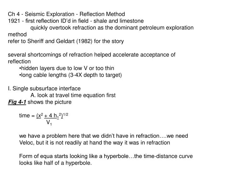
Ch 4 - Seismic Exploration - Reflection Method

1. Ch 4 - Seismic Exploration - Reflection Method • 1921 - first reflection ID’d in field - shale and limestone • quickly overtook refraction as the dominant petroleum exploration method • refer to Sheriff and Geldart (1982) for the story • several shortcomings of refraction helped accelerate acceptance of reflection • hidden layers due to low V or too thin • long cable lengths (3-4X depth to target) • I. Single subsurface interface • A. look at travel time equation first • Fig 4-1 shows the picture • time = (x2 + 4 h12)1/2 • V1 • we have a problem here that we didn’t have in refraction….we need Veloc, but it is not readily at hand the way it was in refraction • Form of equa starts looking like a hyperbole…the time-distance curve looks like half of a hyperbole.

2. Move to Fig 4-3 to observe diff ways to plot time vs distance. • Fig 4C shows conventional style plot… distance on horiz axis, vert axis in time (below the surface) • controlling factor on intensity of reflection is controlled by acoustic impedance, function of both velocity and density • if 1V1 = 2V2, all energy transmitted, no reflection occurs • bigger the diff between these products, the stronger the reflection • B. Analysis of arrival times • turn to the issue of ID’ing reflections from other wave arrivals • Note that reflected wave hyperbola assymptotically approaches a straight line with slope = 1/V1; Fig 4-2c, 4-4b • Makes sense, because both waves travel at V1 • also note that the 2 waves converge as the reflected wave path becomes much closer to (although still slower than) the direct wave

3. C. Now start looking at normal moveout (NMO) defined: “diff in travel-times from a horizontal reflecting surface due to variations in source-geophone distance” I don’t like his pictures …..try these NMO - tx - to to x time x tx x distance

4. D. determining velocity and thickness With the x2-t2 plot method, slope of the plot is 1/V12 Fig 4-8 so you can determine velocity graphically, then solve for thickness: h1 =toV1 2 Example applied to real field data Fig 4-9 how do we proceed? Construct the plot x2-t2 Determine slope 1/V12 solve for V1 solve for h1 II. Multiple horizontal interfaces Fig 4-12.shows that reflection paths are not as simple as we’d like to see, but the Dix equation allows us to determine the rms (average) velocity to each interface

5. A. determining velocity Dix equa allows us to use the x2-t2 plots for multiple layers and velocities We solve for the interval velocity of one layer: start with assumption that Vrms1 = V1 then using the velocities from x2-t2 plot, you use the Dix equation to solve for successive interval velocities (aka Vn) in lower layers Why? Because with interval velocities and times to upper and lower boundaries, we can calculate thicknesses Equa 4-20 fairly forbidding, but not that tough…use the third layer of the example to wade through the symbols.. V32 = Vrms23 to3 - Vrms22 to2 to3 - to2 B. determining thickness - equa 4-22 - use the third layer as example h3 = V3 (to3 - to2) ( 2 )

6. C. More on Dix method (!) • Pages 158-64 spent discussing problems that occur when source-receiver distances get larger…more error introduced into velocity and depth calculations. • At end of section, a real seismogram from Mass is used for analysis using the Burger computer programs…may be a good exercise for us. Note that for both reflectors analyzed, the key to their identification was the tie back to well control. • III. Dipping Interface • As in the refraction case, we can’t merely ID a dipping interface from a one-way shoot…need forward and reverse shots. • One way to achieve this geometry is through a center-shot array (fig 4-19) • Travel time for a dipping interface now determined • housekeeping: x is positive to the right of the source but negative to the left • t = (4j2 + x2 - 4 jx sin )1/2 • V • which is equation for a hyperbola Fig 4-20

7. Hyperbola shows the travel times for both a horiz and dipping interfaces one thing fairly easy to see; on horiz surface, the fastest path is straight down and back up to geophone right at the source… on dipping surface, shortest and fastest path is not straight up and down so geom differences cause the center of hyperbola to appear offset updip A. Determining dip, thickness, and velocity do a little calc, and find value of xmin xmin = 2j sin  and tmin = 2j cos V tmin = cos  to and h = j cos  any of several preceding equations can be used to get V now we know the above

8. B. Turn to another approach for dip, thickness, velocity (p.172) • graphic approach w/ x2-t2 here • 2 diff lines, one each for updip, downdip • plot the average line between the 2 lines, inverse of that slope is V2. • This technique also yields accurate estimates for dip and thickness with eqs 4-26 and 4-37. • C. Normal Moveout again • why here??? • To use it in a final approach for dip, thickness, and veloc determination. • D. Dip moveout approach • defined: diff in t-t to geophones at equal distance from source… • T DMO = t+x - t-x Fig 4-23 • use this info and the V from an x2-t2 plot, with following equation to get : •  = sin-1 (- V T DMO) where x is pt at which you measure T DMO • 2x

9. III. Acquiring and recognizing reflections • Reflection may be a pain in the butt but incentive to produce “great detail” exists • equip design, data processing, and survey design can all help • us ID: 1) similarity of waveform, and 2) exhibition of NMO • A. the Optimum Window • Fig 4-24 used here as data • model parameters shown…4 layers, 3 interfaces@ 5, 30, 50 meters • Water Table reflec at 5m (jump in V below it to 1400m/sec, from 400 m/sec above) • also see a good water table refraction (note the STRAIGHT line response of the refractor, vs the CURVED response of the reflections…this is why ID of NMO character is important on raw seismic sections - differentiate between refractions and reflections • point of Burger is that it may be VERY difficult to determine reflections from real data • one way to counter this is to OFFSET your first receiver further from the source..pushes the low velocity, large waves much further down the section (later in time), distances this “noise” from your reflection and refraction data

10. Thus the optimum window is that source-receiver configuration that pushes your noise “out of the picture”, and allows you to concentrate on your data of interest. • Real-life example presented in Fig 4-26 - note how much clearer the reflections are once the low V noise is pushed down the record • Practical point - what do you do in the field? Time and funds permitting, begin to increase your updip and downdip spread lengths, and “reflections will emerge from the low-velocity waves” (p.187) • B. Multiple reflections • we must consider “non-simple” reflection paths - • thus far we have considered “primary” reflections (source-interface-geophone) • “multiples” are defined as those arrivals that have undergone more than one reflection prior to hitting the geophone • both short- and long-path multiples exist • short path not a separate event..more like a tail • long path can appear as a separate “real” event, often misinterpreted as primary events

11. Obviously, mapping multiples as real events is a mistake in interpretation • so we have to recognize and deal with them • complex method shown to keep track of energy loss…bottom line is that multiples are not usually strong unless there are large velocity contrasts and simple travel paths with few boundaries - these conditions allow multiple energy to persist • in cases where we do have multiples, how can we manage them? • One thing we see is that multiples are twice the travel-time of the primaries Fig 4-28 shows this on x2-t2 plot clearly • so the give-aways to multiples are events that are twice the travel time and less energetic than a primary, and calculated velocity from an x2-t2 line that is same as the primary • multiples a big problem in petroleum, deep reflection data • less of a problem in shallow environmental work

12. IV. Diffractions these develop when seismic waves of a certain wavelength encounter radii of curvature similar to wavelength 100 Hz frequencies in sources usually associated with approx 15 m wavelengths…this sets a stage in our work to encounter diffractions effect of diffractions - can produce non-horizontal reflections that may look like subsurface structures such as anticlines - big problem in deep petroleum exploration, not so much in shallow invironmental work V. Common Field Procedures focus on 3 oprns & geophone spreads after brief review of equipment.. A. Reflection work is all about enhancing the highs 2 reasons: remove low freq noise in order to see the reflection improve resolution in order to see detail Fig 4-31 for the resolution parameters given: 1500m/sec V avg, beds 7.5 m apart

13. 2 seis pulses: 10 m , 150 Hz 20 m , 75 Hz 150 Hz signal shows 2 beds, the 75 Hz does not… some folks say vertical resolution is  /4, but we say  /2 for shallow work horiz resolution dictated by Fresnel zone, the radius of the circle made by the spherical wave when it hits a bed: Wave hits a bed R1 = (1/2  h1)1/2 bottom line…better resolution horiz with high freqs, just like in vert resolution..here, the geophone spacing plays a role too by dictating the sampling interval horizontally

14. Thus good rules of thumb might be:  /2 = vertical resolution geophone spacing/2 = horiz sample interval So how do we get high freqs into and out of the ground? Hammer source, 14 Hz phones with 100 Hz low-cut filters are OK for seeing bedrock but 100 Hz phones, 200 Hz low cut filters and shotgun source can give you detail of stratigraphy above the bedrock one modern trick - use multiple blows to to sum the energy of the signal…. B. Geophone spreads split spread common-offset common-depth-point (CDP)

15. 1. Split spread good for survey at one location start with small offset lets you get refraction data for near-surface velocity then increase your offset until you find the optimum window also determine your best filter..remember that filter may remove too much of your energy needed for interpretation once you start the survey, the phone-source geometry moves around some (Fig 4-32) an actual seismic section can be produced after we remove NMO and “correct for statics” but if we really want seismic sections that cover more ground, we go to a different approach than the split spread 2. Common offset (Hunter et al, 1984) simple, efficient first find the optimum window and optimum offset from source to receiver start your shots E1-G1then , E2-G2 then E3-G3, and so on one shot to one receiver

16. One advantage to common offset is there’s no NMO correction, because no diff between the source-receiver distance along the line Common offset data should be processed. (a whole new area of geophysics!) Examples of the types of data produced are in Fig 4-36, 4-37…. C. Common depth point method