Download
1 / 13
130 likes | 207 Views
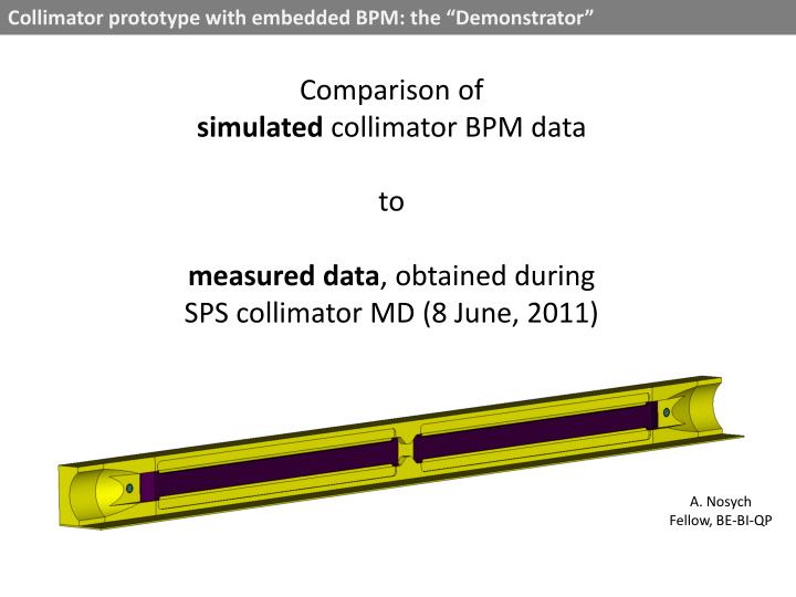
Collimator prototype with embedded BPM: the “Demonstrator”. Comparison of simulated collimator BPM data to measured data , obtained during SPS collimator MD (8 June, 2011). A. Nosych Fellow, BE-BI-QP. Model of the Collimator prototype with embedded BPM: the “Demonstrator”.

E N D
Collimator prototype with embedded BPM: the “Demonstrator” Comparison of simulatedcollimator BPM data to measured data, obtained during SPS collimator MD (8 June, 2011) A. Nosych Fellow, BE-BI-QP
Model of the Collimator prototype with embedded BPM: the “Demonstrator” EM simulation is done with CST Particle Studio Left jaw with BPMs at the ends, middle buttons are not considered in simulation Graphite R4550 r = 13 mWm Copper r = 17 nWm S-steel 316L Special jaw tapering with extrusions to emulate the RF contacts
1. Start of the experiment in SPS Collimator is parked Beam at arbitrary location* (single coasting bunch) *since the vertical beam location is irrelevant, consider the beam somewhere on X axis Jaw gap (D) = 60.8 mm (parked) Button distance (B) = D + 21 mm Bunch length (4sigma) = 2.1 ns Left jaw downstream view Right jaw beam Collimator center
3. Center jaws around beam, move jaws around beam Experiments are done with gaps of [around] D = 28, 24, 20, 16, 12 and 8 mm. Centering is done via microcontroller. Beam position is measured in several locations: at [around] 0%, 20%, 40%, 60% and 80% of each D/2 (half gap size) Exact jaws positions are recorded in Timber at every step. At 8 mm 20% offset the BLMs detect losses and jaws are not moved any closer. D = 28 mm 0% 20% 40% 60% 80% D = 24 mm 0% 20% 40% 60% D = 20mm 0 20 40 60 80% D =16 0 20 40 60% D =12 0 20 40% D =8 0 20%
5. Raw measurement vs. simulation Examples of raw beam position measurement compared to simulation. 80% 60% 60% 40% 40% 20% beam offset 20% beam offset beam centered beam centered Raw measurement can be corrected for initial jaws offset and for electronic offset.
4. Differences between measurement and simulation setup • Measurement errors NOT under control: • Difficult to align jaws at precise positions, keeping constant gap => different geometric setup at every step => imprecise comparison with simulation; • Problems with data transmission from Microcontroller to logging device => unknown error in measured data; • Beam is never parallel to jaws in reality => upstream/downstream measurements lead to different results and must be treated separately; • Real collimator buttons are retracted for extra 0.5 mm from the tapered collimator surface, which adds 1 mm to total button distance (see pictures on right): 21 mm in reality vs. 20 mm in simulations => plays bigger role as jaws get closer. Real collimator 0.5 mm 10 mm 10 mm Model Measurement errors under control: Jaw offset for centered beam (precisely known); Estimated location of electrical center of the linearity characteristic (approximate).
5. Remove initial jaw offset from raw data Raw data correction, step 1: correcting for beam center Given the collimator natural coordinate system (x’,y’) with off-centered beam, Introduce a new coordinate system (x,y) centered around the beam. D Beam centered y´ y xc xR x´ x Collimator center
6. Remove electronics’ offset from raw data Raw data correction step 2: overlay linearity characteristics to have a common “electrical center”: yerr xc Example: Raw and corrected non-linearity of a 28mm gap
7. Measurement vs. simulation. Gaps of 28, 24 and 20 mm Non-linearity of beam position measurement Jaw dist, D = 28 mm 0% 20% 40% 60% 80% Button dist, B = 48 mm D = 24 mm 0% 20% 40% 60% B = 44 mm D = 20mm 0 20 40 60 80% B = 40 mm
7. Measurement vs. simulation. Gaps of 16, 12 and 8 mm Non-linearity of beam position measurement D = 16 mm 0 20 40 60% B = 36 mm D = 12 mm 0 20 40% B = 32 mm D = 8 mm 0 20% B = 28 mm
8. Measurement vs. simulation: slopes Measurement: Up-stream non-linearity slopes (per point) Measurement: Down-stream non-linearity slopes (per point) Simulation: map of slopes vs. button distances, ranging from parked jaws at 60 mm (B=80mm), to operational distance of 2mm (B=22mm) Bad news: linear non-linear non-linear Good news: Both non-linearities can be predicted trough simulation.
9. Conclusion • Conclusion: • Despite the presence of several error sources and imperfections of measurement, a good agreement between simulation and measurement is observed. • Horizontal correction factor is non-linear with respect to jaw gap. • Behavior of real collimator BPM signals for various jaw gaps can be predicted through simulation. • Correction factors can be derived from simulated signals for several jaw gaps and building a fit to cover the whole jaw motion range. Anticipation: Since several major error sources are already understood/eliminated, more collimator BPM MDs are desired throughout 2012 to improve validation of the model. Several short measurements (with several gaps) would be sufficient. Acknowledgements: Marek Gasior, Christian Boccard.
10. Reserved slide Transverse non-linearity maps

![Data Modeling [Comparison of data modeling techniques ]](https://cdn0.slideserve.com/205866/data-modeling-comparison-of-data-modeling-techniques-dt.jpg)


![Data Modeling [Comparison of data modeling techniques ]](https://cdn3.slideserve.com/6795343/data-modeling-comparison-of-data-modeling-techniques-dt.jpg)