Download
1 / 64
660 likes | 840 Views
Controller Design for Dynamically Positioning of Marine Vessels. Professor Asgeir J. Sørensen, Department of Marine Technology, Norwegian University of Science and Technology, Otto Nielsens Vei 10, NO-7491 Trondheim, Norway E-mail: Asgeir.Sorensen@ntnu.no. Outline. Control plant model

E N D
Controller Design for Dynamically Positioning of Marine Vessels Professor Asgeir J. Sørensen, Department of Marine Technology, Norwegian University of Science and Technology, Otto Nielsens Vei 10, NO-7491 Trondheim, Norway E-mail: Asgeir.Sorensen@ntnu.no
Outline • Control plant model • Linear low-frequency vessel model • Linear wave-frequency model • DP Observer • Reference model • Horizontal-plane controller • PD control law based on LQG synthesis • Integral action • Wind feedforward • Model reference feedforward • Pitch and roll motion damping controller • Controller analysis • Thrust allocation
DP Control System Overview THRUSTER SETPOINTS MEASUREMENTS SIGNAL PROCESSING THRUST ALLOCATION REAL WORLD POWER MANAGEMENT SYSTEM POWER LIMITS VESSEL OBSERVER CONTROLLER COMMANDED THRUSTER FORCES VESSEL MOTIONS OPERATOR
Vessel model Superposition, LF + WF
Low-frequency Control Plant Model M D G w X % + X + R = b + thr Hydrodynamic Couplings:
Model reduction matrices Define: Model reduction: T M H MH = i i 6 i 6 × × T Ý Þ D H D D H = + m L i i 6 i 6 × × T Ý Þ G H G G H = + m B i i 6 i 6 × ×
Low-frequency Control Plant Model Linearized low-frequency state-space formulation: • i = 3: surge, sway, and yaw • i = 5:surge, sway, roll, pitch and yaw x A x B E w % = + b + i i i i ic i i y C x v = + i i i i where: T T ß à ß à x u , v , r , x , y , x u , v , q , p , r , x , y , , , = f = d S f 3 5
- (Wind) • Waves • Current • Thruster Losses • Other unopened • slowly-varying effects Bias model (Markov model) Low-frequency Control Plant Model 3 DOF Vessel model (Low Speed) Tb may be set equal to 0 (Wiener model).
Wave-frequency Control Plant Model Synthetic white-noise-driven wave-frequency state-space formulation for i = 3 DOF horizontal model: % A E w Y = Y + 3 w 3 w 3 w 3 w 3 w C R = Y 3 w 3 w 3 w where: T ß à x , y , 6 3 R R = f R 5 w 5 Y w w w 3 w 3w 3 w á â diag , , I = g g g á â K diag K , K , K á â = diag , , C = Q Q Q 1 2 3 w w 1 w 2 w 3 1 2 3 This corresponds to three decoupled WF models on the form: K s R Ý Þ w s w = i i w 2 2 w s 2 s i + Q g + g i i i
Wave-frequency Control Plant Model Synthetic white-noise-driven wave-frequency state-space formulation for i = 3 DOF horizontal model and i = 5 DOF model: % A E w Y = Y + iw iw iw iw iw C R = Y iw iw iw where:
Wave-frequency Control Plant Model WF model Example: 2nd order WF model (notch-filter)
Resulting Control Plant Model Wave-frequency model: Low-frequency ship dynamics: Bias model accounting for un-modeled dynamics and slowly varying disturbance: Kinematics: Measurements:
Model Uncertainties • Vessel Speed • Wave response • Coupling effects and parameters in M and D • Degree / linearization of model • Thruster losses (direction / thrust) • Wave period (peak frequency) Note ! Error in measurement can often be a significant contributor to reduced system performance !
Discretization of model: Extended Kalman Filter
Ý Þ R f Extended Kalman Filter Predictor: Corrector: • Time-varying Kalman filter gain only because of • Tuning of Kalman filter gain via Q and R matrices • intuitive / related to physics ? • ”noise” focused design
Nonlinear Observer Observer Detailed ship model Weighted, quality checked position and heading measurements Model adaptation • Purpose: • Noise filtering • Wave filtering • Estimates of vessel positions and velocities • Dead reckoning Filtered estimates used by the feedback controller
x A x A x % = + Ý Þ x A x H J A x % = + 1 1 1 1 1 2 2 1 1 1 1 1 2 2 Separate kinematics from the other parts of the model x % A x A x = + ? 1 Ý Þ x % A H J x A x = + 2 2 1 1 2 2 2 2 2 1 1 2 2 2 A nonlinear approach Is it possible to design a linear observer and afterwards extend local results to a global setting by inserting rotations? Under what conditions may the rotations be removed from the stability analysis?
WF LF Body-Fixed Earth-fixed x A x E w % = + w w w w w Ý Þ R R % = f X y % ? 1 ? b T b E w = + b b b T T ? Ý Þ ? Ý Þ M GR D R b X % = f R X + b + f y y x T T Ý Þ AT Ý Þ x B Ew % = f f + b + y y T T Ý Þ Ý Þ T diag R Ý Þ , . . , R Ý Þ , I f = f f y y y Nonlinear Observer Compact Formulation:
Ý Þ p Ý Þ cos cos f + f f w Ý Þ p Ý Þ sin sin f + f f w Model Properties / Assumptions Assumptions for stability analysis of Observer: 1. Used in passivity-based design of nonlinear observer 2. Bounded WF part of heading motion (e.g. less than 5 degrees)
Nonlinear Observer (Basic version) Observer
Observer Error Dynamics Control Plant Model Observer equations Error dynamics
T T V x P x M 0 * * * * = + X X > o o % T T Ý Þ V x PA A P x * * = + o o o o T T ? Ý Þ D D * * X + X + T T Ý Þ 2 R B P x * * + X f y o o T T Ý Þ 2 R C x * * + X f y o o T 2 x PE w * + o o % T T T T ? ? Ý Þ V x Q x D D 2 x PE w * * * * * = X + X + o o o o % ? 1 V 0 , x 2 Q E w * q q q q < > o o Lyapunov Analysis KYP Lemma ISS / GES
K , K , K , K 1 2 3 4 Stability Requirements Stability Requirement: Choose Such that
Loop Shaping of Error Dynamics Fase > -90 deg = passive
0 0 -20 -10 [dB] [dB] y -20 -40 ! Ì R -30 -60 -40 -80 -3 -3 -2 -2 -1 -1 0 0 1 1 2 2 10 10 10 10 10 10 10 10 10 10 10 10 Frequency [rad/s] Frequency [rad/s] y ! Ì X 2 / T g = ^ o p Loop Shaping 1st order wave loads
Adaptive Control Systems • Some kind of ’adaptiveness’ present in most hi-tech • Marine systems today (observer / controller): • Gain Scheduling (robust) wrt. • Operation • External measurements • Operations • Model-predictive control (MPC) • Online adaptive observers / controllers Examples: Autopilots, DP systems
Adaptive Observer WF model WF model parametrization: Assumed constant parameters in stability analysis (of course not entirely true …)
Adaptive Observer Purpose: Compute online the WF model parameters that Matches the WF motion of the vessel. Adaptive version of WF update law: High-pass filtered
Error Dynamics –Adaptive Observer WF model error dynamics ”After some algebra….” Total error dynamics: KYP / SPR requirements:
Experimental Tests – GNC Lab 1999 Cybership I
Reference Model Reference model of third order: e e e a v x x + I + @ = @ ref d d d x ? A x A % = + R ref f ref f r Where the final Earth-fixed position and heading are given by: In reference parallel frame the desired position and heading are given by:
Reference Model Reference model of third order: Where the final Earth-fixed position and heading are given by: Optimal Earth-fixed position and heading are given by: is the optimal vessel increment subject to some criteria
Controller Design - LQG Feedback Performance index defined to compute Linear-Quadratic-Gaussian feedback controller in surge, sway and yaw accounting for i = 3 DOF horizontal model and i = 5 DOF model: T X 1 T T J E lim e Qe P dt = + b b T K pd ¸ pd T 0 Deviation vector is defined to be: Ricatti equation: Let: LQG Feedback Control law is: ? G e ? G e b = p 2 1 pd d
Controller Design - Resulting Control Law LQG feedback control law is: ? G e ? G e b = p 2 1 pd d Integral action: A G e b % = b + wi i i 2 i Wind feedforward control action: ? G b = ! b w wind w Reference model feedforward control action: Ý Þ Ý Þ M a D v d v C v v b = + + + 3 3 3 d d d d d t Resulting feedback and feedforward control law is: b = b + b + b + b w t 3 c i pd
Positioning with Roll, Pitch Damping • Hydrodynamic coupling between: • Surge and pitch • Sway, roll and yaw • Geometrical coupling by thruster configuration: • Thruster induced pitch moment due to surge positioning • Thruster induced roll moment due to sway and yaw positioning • Resonance periods in roll and pitch in the range of 35-65 s: • within bandwidth of positioning controller
Controller Design - Resulting Control Law Roll-pitch damping controller: where Resulting positioning controller with roll-pitch damping: b = b + b 5 c 3 c rpd
Thrust allocation M D G w X % + X + R = b + ic Relation between 3 DOF control vector - surge, sway and yaw and r number of thruster/propellers is: Ý Þ T Ku b = J 3 r c ic × Thrust produced by each propeller: 1 Ý Þ ? + u K T + = J b Ý Þ Ku T = J b c ic 3 r c × 3 r ic × Real thrust acting on the vessel in 6 DOF: Ý Þ T Ku b = J 6 r c × thr
Thrust allocation Aziumuthing thrusters 1. Bow azimuthing thruster lba 2. Bow tunnel thruster Surge lbt Yaw Sway lst 3. Stern tunnel thruster lp bp bs 4. Starboard pod 5. Port pod
Wave Frequency • Current loads • Wind loads • 2nd order wave loads Low Frequency 1st order wave response Thrustersetpoints ThrusterAllocation Controller Vessel Observer Actual positions,velocities Sensors Measurements Reference Model Operator High Level Plant Control
Transfer Function from Disturbance in Surge to Pitch Angle Magnitude [dB] 0 -20 -40 -60 Open Loop Closed Loop 3 DOF Closed Loop 5 DOF -80 0 0.005 0.01 0.015 0.02 0.025 0.03 Frequency [Hz]
Transfer Function from Disturbance in Pitch to Pitch Angle Magnitude [dB] 0 -10 -20 -30 Open Loop Closed Loop 3 DOF -40 Closed Loop 5 DOF 0 0.005 0.01 0.015 0.025 0.02 0.03 Frequency [Hz]
Transfer Function from Disturbance in Roll to Roll Angle Magnitude [dB] 0 -10 -20 -30 -40 Open Loop Closed Loop 3 DOF Closed Loop 5 DOF -50 0 0.005 0.01 0.015 0.02 0.025 0.03 Frequency [Hz]
Coupled Dynamics Surge-Pitch Dynamics: Surge Control Law: Pitch damping Closed-Loop pitch dynamics: X, U -> 0 by control
DP with Roll and Pitch Damping - Time Series Surge [m] 0.2 • Wave: • Hs = 6 m • Tp = 10 s • wave = 225 deg • Current: • Vcur = 0,5 m/s • cur = 225 deg • Wind: • Vwind = 10 m/s • wind = 225 deg 0 -0.2 -0.4 0 200 400 600 800 1000 Pitch [deg] 0.4 With roll-pitch damping No roll-pitch damping 0 -0.4 -0.8 0 200 400 600 800 1000 time [sec]
DP with Roll and Pitch Damping - Time Series Thrust in surge [kN] 600 400 • Wave: • Hs = 6 m • Tp = 10 s • wave = 225 deg • Current: • Vcur = 0,5 m/s • cur = 225 deg • Wind: • Vwind = 10 m/s • wind = 225 deg 200 0 0 200 400 600 800 1000 Thruster induced moment in pitch [kNm] 4 x 10 2.5 With roll-pitch damping No roll-pitch damping 2 1.5 1 0.5 0 0 200 400 600 800 1000 time [sec]
DP with Roll and Pitch Damping - Time Series Sway [m] 0.5 0 • Wave: • Hs = 6 m • Tp = 10 s • wave = 225 deg • Current: • Vcur = 0,5 m/s • cur = 225 deg • Wind: • Vwind = 10 m/s • wind = 225 deg -0.5 -1 Roll [deg] 1 0.5 0 -0.5 Heading [deg] With roll-pitch damping 0.1 No roll-pitch damping 0 -0.1 0 200 400 600 800 1000 time [sec]