Download
1 / 46
460 likes | 527 Views
High Speed Stable Packet Switches. Shivendra S. Panwar Joint work with : Yihan Li, Yanming Shen and H. Jonathan Chao New York State Center for Advanced Technology in Telecommunications (CATT) Electrical and Computer Engineering Dept. Polytechnic University, New York

E N D
High Speed Stable Packet Switches Shivendra S. Panwar Joint work with: Yihan Li, Yanming Shen and H. Jonathan Chao New York State Center for Advanced Technology in Telecommunications (CATT) Electrical and Computer Engineering Dept. Polytechnic University, New York http://catt.poly.edu/CATT/panwar.html
Overview • Switching technology continues to be one of the bottlenecks in the development of broadband networks • Fixed-length switching technology achieves high switching efficiency for high-speed packet switches • Virtual Output Queueing (VOQ) switches can achieve 100% throughput without speedup • Two approaches to resolve the output contention in a VOQ switch • Matching algorithms • Load-balanced switch • Switch performance • Throughput • Packet delay
1 1 1 1 2 2 2 2 3 3 3 3 4 4 4 4 Buffering in a Packet Switch • High speed fixed-length packet switching • Input Queuing (IQ) • Easy to implement • HOL Blocking, throughput 58.6% • Output Queuing (OQ) • 100% throughput • Internal speedup of N • Virtual Output Queuing (VOQ) • Overcome HOL blocking • No speedup requirement
Matching Algorithms • Scheduling in a VOQ switch • Stable matching schemes for VOQ switching • Maximum Weight Matching (MWM) • Maximal Matching, iSLIP • Other algorithms with 100% throughput and no speedup • Polling system based matching • Exhaustive Service Matching with Hamiltonian Walk • Limited Service Matching • Average delay analysis
Scheduling in a VOQ Switch • Scheduling is needed to avoid output contention. • A scheduling problem can be modeled as a matching problem in a bipartite graph. • An input and an output are connected by an edge if the corresponding VOQ is not empty. • Each edge may have a weight, which can be • The length of the VOQ • The age of the HOL cell
Maximum Weight Matching (MWM) 7 • MWM always finds a match with the maximum weight • Complexity of O(N3). • Is stable with 100% throughput under all admissible traffic. 4 3 7 8 5 6 10 5 2 Weight of the match: 25
Maximal Matching 7 • Maximal Matching • Add connections incrementally, without removing connections made earlier. • No more matches can be made trivially by the end of the operation. • Stable with a speedup of 2 • Complexity O(NlogN) • Multiple Iterative Matching • Use multiple iterations to converge to a maximal matching • iSLIP and DRRM • complexity of each iteration is O(logN) • O(logN) iterations are needed to converge on a maximal matching 4 3 7 8 5 6 10 5 2 Weight of the match: 23
iSLIP Output • Step 1:Request • Each input sends a request to every output for which it has a queued cell. • Step 2:Grant • If an output receives multiple requests it chooses the one that appears next in a fixed round-robin schedule. • The output arbiter pointer is incremented by one location beyond the granted input if, and only if, the grant is accepted in step 3. • Step 3:Accept • If an input receives multiple grants, it accepts the one that appears next in a fixed round-robin schedule. • The input arbiter pointer is incremented by one location beyond the accepted output. Input Request Grant Accept
Achieving 100% Throughput without Speedup • Algorithms with memory • [Tassiulas] Compare the latest schedule to a randomly generated match, select the one with higher weight as the new match, complexity O(logN). • [Giaccone et al] • Derandomized algorithm, using Hamiltonian walk, complexity O(logN). • Other algorithms, with higher complexity, take into account the latest schedule, its neighbors, and the arrival pattern. • SERENA, complexity O(N). • Polling system based matching algorithms • Low complexity: HE-iSLIP, O(logN). • Low packet delay • Much lower than other O(logN) algorithms. • Comparable to higher complexity algorithms.
ORM VOQ ISM 1 Input 1 Switch Fabric Output 1 N 1 1 1 1 1 N N N N Input 2 Output 2 N 1 Input 3 Output 3 N 1 Input 4 Output 4 N The Architecture of a Cell-Based VOQ Switch • Previous work • Try to find a good match in each (cell) time slot. Cells in the same packet are interrupted during transmission. • Considered cell delay, not packet delay. Input Segmentation Module (ISM):Segment packets to fixed-length cells. Output Reassembly Module (ORM):Reassemble cells into packets.
Polling System Based Matching • Exhaustive Service Matching • Inspired by exhaustive service polling systems. • All the cells in the corresponding VOQ are served after an input and an output are matched. • Slot times wasted to achieve an input-output match are amortized over all the cells waiting in the VOQ instead of only one. • Cells within the same packet are transferred continuously. • Hamiltonian walk is used to guarantee stability. • Hamiltonian walk is a walk which visits every vertex of a graph exactly once. • For an NxN switch, each possible match is visited exactly once in every N! time slots.
Exhaustive Service Matching with Hamiltonian Walk (EMHW) • EMHW • Let S(t) be the match at time t. • At time t+1, generate match Z(t+1) by the Exhaustive Service Matching algorithm based on S(t), and H(t+1) by Hamiltonian walk. • Let where <S,Q(t+1)> is the weight of S at time t+1. • Stability Theorem 2:An EMHW is stable under any admissible Bernoulli i.i.d. input traffic.
Implementation Complexity of EMHW • Implementation complexity • EMHW: O(logN) for HE-iSLIP • HE-iSLIP: only one iteration is needed to achieve 100% throughput and low packet delay. • Compare to the Derandomized Matching Algorithm (O(logN)) • The weight of the schedule generated by EMHW is always larger than or equal to the schedule generated by the derandomized matching algorithm. Theorem:Suppose the schedule at time t is M(t), and at time t+1 the schedule by the derandomized matching algorithm and EMHW are Sd(t+1) and S(t+1), respectively. Then it is always true that
Limited Service Matching • An approximation to EMHW with lower complexity. • When a VOQ is under service, a limit on the maximum number of cells that can be served continuously is enforced by means of a counter. • No Hamiltonian walk is used. • Limited Service Matching DRRM can be implemented in a distributed manner.
1 1 1 1 N N N N ORM VOQ ISM 1 Input 1 Switch Fabric Output 1 N 1 Input 2 Output 2 N 1 Input 3 Output 3 N 1 Input 4 Output 4 N Simulated Delay Performance • Packet delay: the sum of cell delay and reassembly delay • Cell delay: measured from VOQ to destination output • Reassembly delay: time spent in an ORM, often ignored in other work.
Traffic Patterns in Simulations • Uniform traffic • Pattern 1: packet size is 1 cell. • Pattern 2: packet size is 10 cells. • Pattern 3: packet size is varied and the average is 10 cells (Internet packet size distribution). • Nonuniform traffic • Diagonal traffic, packet size is 1 cell. • Hotspot traffic, packet size is 1 cell.
Packet Delay under Uniform Traffic • Pattern 1: packet size is 1 cell. SERENA iSLIP HE-iSLIP MWM
Packet Delay under Uniform Traffic • Pattern 3: packet length is variable, the average is 10 cells. • Pattern 2: packet length is 10 cells. SERENA SERENA iSLIP MWM iSLIP MWM HE-iSLIP HE-iSLIP
HE-iSLIP MWM MWM HE-iSLIP When Packet Length is Larger Than 1 Cell • Why does HE-iSLIP have a lower packet delay than MWM? • For example, when packet length is 10 cells: • Reassembly delay • Cell delay • Low cell delay and low reassembly delay needed for low packet delay
Performance Analysis-- Average Delay of E-iSLIP (1) • Exhaustive random polling system model • Symmetric system -- only consider one input • N VOQs per input, exhaustive service policy -- an exhaustive service polling system with N stations • The service order of the VOQs are not fixed -- random polling system, assume all station VOQs have the same probability of selection for service after a VOQ is served.
Performance Analysis-- Average Delay of E-iSLIP (2) • Switch over time S • Average delay T [Levy]
Performance Analysis-- Average Delay of E-iSLIP (3) • When N is large
EMHW Summary • Exhaustive Service Matching with Hamiltonian walk (EMHW) • Stable under any admissible Bernoulli i.i.d. input traffic. • HE-iSLIP, complexity O(logN) • Packet delay performance • Compared to iSLIP (O(logN)), Derandomized Algorithm (O(logN)), SERENA (O(N)) and MWM (O(N3)), under uniform traffic, • HE-iSLIP has lower packet delay than the Derandomized algorithm and SERENA. • HE-iSLIP has lower packet delay than MWM for typical packet sizes. • HE-iSLIP has low cell delay and low reassembly delay, which lead to low packet delay.
Load-Balanced Switches • Switch architecture • Packet out-of-sequence issue • Packet scheduling in the first-stage switch • Packet delay performance • Conclusions
Motivation • Challenges in designing high-performance switch • Scalable • Scale to high number of linecards and to high linecard speeds • No centralized scheduler • Low complexity • Provide performance guarantees • 100% throughput guarantee • no commercial switch today has a throughput guarantee. • Load-balanced switch • 100% throughput for broad class of traffic • No centralized scheduler needed, scalable
Work on Load-balanced Switches • Original load-balanced switch (Computer Communications, Chang) • 100% throughput • Unbounded out-of-sequence delay • FCFS (First come first serve) (Computer Communications, Chang) • Jitter control mechanism • Increases the average delay • EDF (Earliest deadline first) (Computer Communications, Chang) • Reduce the average delay • High complexity • Mailbox switch (Infocom 2003, Chang) • Prevents packets from being out-of-sequence • Not 100% throughput • FFF (Full frames first) (Infocom 2002, Mckeown) • Frame-based • No need for resequencing • Require multi-stage buffer communication • FOFF (Full ordered frames first) (Sigcomm 2003, Mckeown) • Frame-based • Maximum resequencing delay N2 • Bandwidth wastage
1 … N N N … … … i 2 2 2 1 1 1 … N ... ... ... ... ... ... ... ... ... ... ... ... Byte-Focal Switch Architecture Re-sequencing buffer 1st stage switch fabric 2nd stage switch fabric Arrival Input VOQ Second-stage VOQ (1,1) (1,1) 1 1 1 (1,k) (1,k) (1,N) (1,N) … … (i,1) (j,1) … j k i (j,k) (i,k) (j,N) (i,N) … … (N,1) (N,1) … (N,k) N N (N,k) N (N,N) (N,N)
Switching fabric • Deterministic and periodic connection pattern • At both stages, at time slot t, input i is connected to output j with j = (i+t) mod N t=0 t=1 t=2 t=3
Load-Balancing Second stage VOQ (1,k) 1st stage switch fabric 2nd stage switch fabric (2,k) (3,k) First stage VOQ(i,k) . . . Packets are sent in Round-Robin order to the second-stage (N,k)
At time t+ Out-of-Sequence Problem 2nd stage switch fabric 1st stage switch fabric ith input port At time t jth central buffer … 2 1 1 1 2 (j+1) th central buffer 2 Maximum re-sequencing delay=N2
1 … N N N … … … i 2 2 2 1 1 1 … N ... ... ... ... ... ... ... ... ... ... ... ... Resequencing Buffer Design Re-sequencing buffer Arrival Input VOQ 1st stage switch fabric Second-stage VOQ 2nd stage switch fabric (1,1) (1,1) 1 1 1 (1,k) (1,k) (1,N) (1,N) … … (i,1) (j,1) … j k i (j,k) (i,k) (j,N) (i,N) … … (N,1) (N,1) … (N,k) N N (N,k) N (N,N) (N,N) Resequencing buffer design
The next packet via center stage queue j has not arrived The HOF packet arrived The index joins the departure queue For i2, j2 is the HOF packet, then the index also joins the departure queue Resequencing Buffer Design … j1 j1+1 Input port i1 j1+2 … . . . . . . i2 i1 Departure queue … j2 j2+1 Input port i2 j2+2 …
1 … N N N … … … i 2 2 2 1 1 1 … N ... ... ... ... ... ... ... ... ... ... ... ... First Stage Scheduling Re-sequencing buffer Arrival Input VOQ Switch fabric Second-stage VOQ Switch fabric (1,1) (1,1) 1 1 1 (1,k) (1,k) (1,N) (1,N) … … (i,1) (j,1) … j k i (j,k) (i,k) (j,N) (i,N) … … (N,1) (N,1) … (N,k) N N (N,k) N (N,N) (N,N) First stage scheduling algorithms
First Stage Scheduling Choose an eligible cell 1st stage switch fabric 2nd stage switch fabric Arbiter At time t, i connected to j … … Up to N HOL eligible cells jth input port of 2nd stage input port i Eligible cells: cells that can be sent to jth input port of 2nd stage Problem: Which VOQ to serve?
First Stage Scheduling • Round-robin • The arbiter at each input port selects VOQs in round-robin order • Unstable under non-uniform traffic • Longest queue first • The arbiter at each input port chooses to serve the longest queue • High complexity, not practical • Fixed threshold scheme • Set a threshold, N, a queue exceeds the threshold has a higher priority • Serve the high priority queue first • Dynamic threshold scheme • Set the threshold as TH=Q(t)/N • Then same as fixed threshold scheme Longest queue first, fixed threshold and dynamic threshold schemes have been proved to be stable in our work.
Simulation Settings • Uniform i.i.d: • Diagonal i.i.d: , for j = (i +1) mod N. This is a very skewed loading, since input i has packets only for outputs i and (i + 1) mod N • Hot-spot: , , for i≠j.This type of traffic is more balanced than diagonal traffic, but obviously more unbalanced than uniform traffic
Average Cell Delay • At the low load, 2-stage switching has larger delay than iSlip, but smaller at high load • FOFF shows large delay even at low load due to the bandwidth waste when transferring partial frames Average delay under uniform traffic with switch size of 32 LQF: Longest queue first FOFF: Full order frame first
Dynamic Threshold • The LQF scheme has the best delay performance • not practical due to its high implementation complexity • Dynamic threshold scheme performance is comparable with the LQF scheme • Compared with fixed threshold scheme, adapt to the non-uniform input loadings, thus achieving a better delay performance, while maintaining low complexity • Focus on the dynamic threshold scheme from now on
Dynamic Threshold • As the input traffic changes from uniform to hotspot to diagonal (hence less balanced), the dynamic threshold scheme can achieve good performance, especially for the diagonal traffic. • The Byte-Focal switch performs load-balancing at the first stage, thus achieving good performance even under extreme non-uniform traffic The average delay of the dynamic threshold scheme under different input traffic patterns with a switch size of 32
Delays with Different Switch Sizes • The average delays are almost linearly dependent on the switch size.
3-stage Delays • 3 delay components: - first stage queueing delay - second stage queueing delay - resequencing delay • The first stage queueing delay and the second stage queueing delay are comparable • The resequencing delay is much smaller compared to the other two delays. The three components of the total delay with switch size of 32
Variable Size Packet Scheduling • Two approaches: • Cell-mode and packet-mode • The average delay is the same • Combining the packet mode scheduling and the dynamic threshold scheme - the packet mode dynamic threshold algorithm: • At each time slot, if it is in the middle of a packet, keep serving this queue • If not, apply the dynamic threshold scheme • The resequencing delay and the reassembly delay overlap • The sum of the resequencing delay and the reassembly delay is bounded by where is the maximum packet length • The additional delay due to packet reassembly is reduced
Packet Delay • Used Internet packet length distribution: trimodal distribution • As with the cell delay, the delay performance is not degraded under non-uniform traffic
Packet Delay • Packet delays increase as the packet length increases, also increases with packet length variance • But with a weak dependence
Conclusion • The maximum resequencing delay is N2 • The dynamic threshold scheme is practical and has good delay performance • The time complexity of the resequencing buffer is O(1) • Does not need communications between linecards • Achieve a uniformly good delay performance over a wide range of traffic matrices • Achieves good performance with low complexity