Download
1 / 48
480 likes | 610 Views
CSE 599 Lecture 2. In the previous lecture, we discussed: What is Computation? History of Computing Theoretical Foundations of Computing Abstract Models of Computation Finite Automata Languages The Chomsky Hierarchy Turing Machines. Overview of Today’s Lecture. Universal Turing Machines

E N D
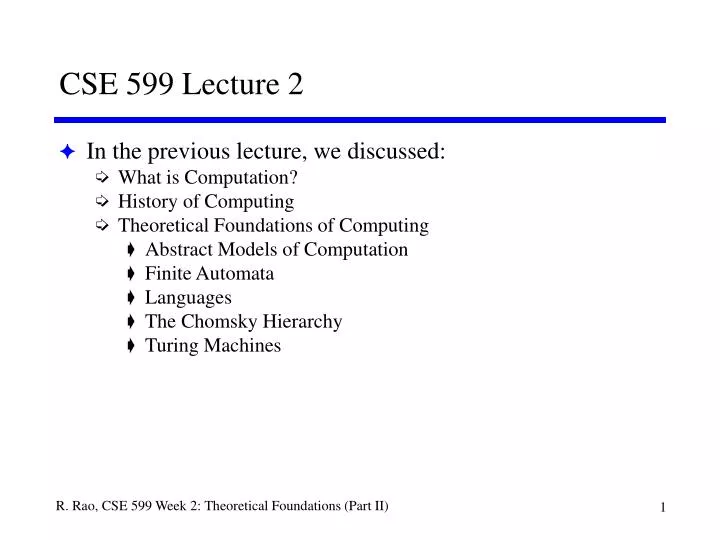
CSE 599 Lecture 2 • In the previous lecture, we discussed: • What is Computation? • History of Computing • Theoretical Foundations of Computing • Abstract Models of Computation • Finite Automata • Languages • The Chomsky Hierarchy • Turing Machines
Overview of Today’s Lecture • Universal Turing Machines • The Halting Problem: Some problems cannot be solved! • Nondeterministic Machines • Time and Space Complexity • Classes P and NP • NP-completeness: Some problems (probably) cannot be solved fast (on classical sequential computers)!
Recall from last class: Turing Machines • Can be defined as a “program”: • (current state, current symbol) to (next state, new symbol to write, direction of head movement), or • A list of quintuples • (q0, s0, q1, s1, d0) • (q1, s1, q2, s2, d1) • (q2, s2, q3, s3, d2) • (q3, s3, q4, s4, d3) • (q4, s4, q5, s5, d4) • etc. • Includes an initial state q0 and • A set of halting states (for example, {q3, q5})
Turing Machines • Example: (q0, 1, q1, 0, R)
Universal Turing Machines (UTMs) • A UTM is a “programmable” Turing machine that can simulate any TM - it is like an interpreter running a program on a given input • Takes as input a description or “program” (list of quintuples) of a TM and the TM’s input, and executes that program • Uses a fixed program (like all TMs) but this program specifies how to execute arbitrary programs • Analogous to a digital computer running a program; in fact, Von Neumann’s stored program concept was partly motivated by UTMs
Universal Turing Machines – How They Work • A UTM U receives as input a binary description of • an arbitrary Turing machine T (list of quintuples) and • contents of T’s tape (a binary string t). • U simulates T on t using a fixed program as follows: • INITIALIZE: copy T’s initial state and T’s initial input symbol to a fixed “machine condition” (or workspace) area of the tape • LOCATE: Given T’s current state q and current symbol s: Find the quintuple (q, s, q’, s’, d) in the description of T; If q not found, then halt (q is a halt state); else • COPY: Write q’ in workspace and s’ in T’s simulated tape region; Move T’s simulated head according to d Read new symbol s’’ and write it next to q’ in workspace • REPEAT: Go to 2.
Universal Turing Machines – Diagram • See Feynman text, Figure 3.23 • This machine uses 8 symbols and 23 different states • Exercise: Identify which portions of the machine executes which subroutine (LOCATE, COPY, etc.)
Now we are ready for the big question… • Are there computational problems that no algorithm (or Turing Machine) can solve? • Surprising answer – YES! • Proof relies on self-reference: UTMs trying to solve problems about themselves. • Related to the paradox: “This sentence is false” • Can you prove the above statement true or false? • Related to Cantor’s proof by “diagonalization” that there are more real numbers than natural numbers
Proof by diagonalization: An example • Show that there are more real numbers than natural numbers • Proof: Form a 1-1 mapping from natural numbers to reals, and form a new real number by changing the ith digit of the ith real number: For example, if 1-1 map is given by: New Real Number = 0.2404……. (Add 1 to diagonal) This number is different from all the ones listed
The Halting Problem and Undecidability • Question: Are there problems that no algorithm can solve? • Consider the Halting Problem: Is there a general algorithm that can tell us whether a Turing machine T with tape t will halt, for any given T and input t? • Answer: No! • Proof: By contradiction. Suppose such an algorithm exists. Let D be the corresponding Turing machine. Note that D is just like a UTM except that it is guaranteed to halt: • D halts with a “Yes” if T halts on input t • D halts with a “No” if T does not halt on input t
Diagram of Halting Problem Solver D • Input to D: description dT of a TM T and its input data t
Diagram of New Machine E • Define E as the TM that takes as input dT, makes a second copy in the adjacent part of the tape, and then runs D:
Diagram of final machine Z (the “diagonalizer”) • Consider the machine Z obtained by modifying E as follows: • On input dT: if E halts with a “No” answer, then halt if E halts with a “Yes” answer, then loop forever • What happens when Z is given dZ as input?
The machine D cannot exist! • By construction, Z halts on dT if and only if the machine T does not halt on dT • Therefore, on input dZ: • Z halts on dZ if and only if Z does not halt on dZ • A contradiction! • We constructed Z and E legally from D. So, D cannot exist. The halting problem is therefore undecidable. • Conclusion: There exist computational problems (such as the halting problem) that cannot be solved by any Turing machine or algorithm.
Computability • We can now make a distinction between two types of computability: • Decidable (or recursive) • Turing Computable (or partial recursive/recursively enumerable) • A language is decidable if there is a TM that accepts every string in that language and halts, and rejects every string not in the language and halts. • A language is Turing computable if there is a TM that accepts every string in that language (and no strings that are not) • Are all decidable languages Turing computable? • Are all Turing computable languages decidable?
Examples: Decidable Languages • The language 0n1n is decidable: • If the tape is empty, ACCEPT • Otherwise, if the input does not look like 0* 1*, REJECT • Cross off the first 0. Then move right until the first 1 (not crossed off) • Cross off that 1, then move left until the first 0. • Repeat the above 2 steps until we run out of 0’s or 1’s • If there are more 0’s than 1’s REJECT • If there are more 1’s than 0’s REJECT • If there are an equal number, ACCEPT • L = { 1n | n is a composite number } is decidable • All decidable languages are Turing computable. Are there Turing computable languages that are not decidable?
Examples: Turing Computable Languages • The Halting Problem is Turing Computable: • HALT = { <dT,t > | dT is a description of TM T, and T halts on input t} • Proof Sketch: The following UTM H accepts HALT • Simulate T on input t. • If T halts, then ACCEPT • Crucial Point: H may not halt in some cases because T doesn’t, but if T does halt, so does H. So L(H) = HALT. • Hilbert’s 10th problem: Given a polynomial equation (e.g. 7x2-5xy-3y2+2x-11=0, or x3+y3=z3), give an algorithm that says whether the equation has at least one integer solution. • Try all possible tuples of integers. • If one of the tuples is a solution, ACCEPT
Beyond Turing Computability • Are there problems that are even harder than HALT i.e. that are not even Turing Computable? • Consider the language DOESN’T-HALT = {<dT,t> | T does not halt on input t} • Result: DOESN’T HALT is not Turing Computable! • Proof: Suppose DOESN’T-HALT was Turing computable and a Turing Machine DH accepts it. Let H be our UTM that accepts HALT. • Define another TM D as follows: On input <dT, t>: • Run H and DH simultaneously (alternate step by step) • If H accepts, ACCEPT • If DH accepts, REJECT • Then D decides HALT! A contradiction, therefore DH does not exist and DOESN’T-HALT is not Turing Computable.
Discussion • THERE ARE PROBLEMS WE JUST CAN’T SOLVE!!! • Software verification is impossible without restrictions • You can’t get around this, but you can reduce the pathological cases • Be careful-- these pathological cases won’t go away • There are mathematical facts we can’t prove: • Gödels Theorem: Any arithmetic system large enough to contain Q (a subset of number theory) will contain unprovable statements • Based on constructing the statement: “This statement is unprovable” • Uses numerical encodings of statements (called Gödel numbers) like those for a TM • Any sufficiently complex system will have holes in it.
5-minute break… Next: Nondeterministic Machines, Time and Space Efficiency of Algorithms
Nondeterminism • We have seen the limitations of sequential machines that transition from one state to another unique state at each time step. • Consider a new model of computation where at each step, the machine may have a choice of more than one state. • For the same input, the machine may follow different computational paths when run at different times • If there exists any path that leads to an accept state, the machine is said to accept the input • Simple Example: NFA (Nondeterministic Finite Automata)
NFA Example • Here’s one example: • There is only one nondeterministic transition in this machine • What strings does this machine accept? • Are NFAs more powerful than DFAs?
NFAs and DFAs are equivalent! • The models are computationally equivalent (the DFA has exponentially more states though in this sketch) • Proof sketch: • each state of the DFA represents a subset of states in the NFA • What about Nondeterministic Turing machines?
Nodeterministic Turing Machines (NTMs) • NTMs may have multiple successor states, e.g. • (q,s,q1,s1,d1) and (q,s,q2,s2,d2) • NTMs are equivalent in computational power to deterministic TMs! • Proof sketch: • Design a machine based on a Universal TM U to simulate NTM M • When there is a nondeterministic transition: (q,s,q1,s1,d1) and (q,s,q2,s2,d2), • U alternates between simulating one computation path and the other (similar to “breadth first search”) • If one of the paths halts, the U halts (with M’s output on its tape) • Nondeterminism useful for time and space complexity issues
Time and Space Efficiency • The fact that a problem is decidable doesn’t mean it is easy to solve. • We are interested in answering: what problems can/cannot be efficiently solved? • Time complexity (worst case run time) is a major concern • Space complexity (maximum memory utilized) is a second concern • We first need to define how to measure the time and space complexity of an algorithm or a TM
Time and Space Complexity of an Algorithm • Example Problem DUP: Given an array A of n positive integers, are there any duplicates? • For example, A: 34, 9, 40, 87, 223, 109, 58, 9, 71, 8 • An easy algorithm for DUP: • for i = 1 to n-1 • for j = i+1 to n • if A[i] = A[j] • Output i and j • Halt • else continue • Space complexity: n + 2 • Time complexity: How many steps in the worst case?
Time and Space Complexity of an Algorithm • An easy algorithm for DUP: • for i = 1 to n-1 • for j = i+1 to n • if A[i] = A[j] • Output i and j • Halt • else continue • Time complexity: How many steps in the worst case? • Worst case = last two numbers are duplicates • Total time steps = • [1 + 3(n-1)] + [1 + 3(n-2)] + … upto n-1 terms • = approximately n2 • = O(n2) (on the order of n2)
“Big O” notation for expressing complexity • A function f(n) is big O of a function g(n), i.e. f(n) = O(g(n)), if there exists an integer N and constant C such that • f(n) c·g(n) for all n N • Thus, our algorithm uses O(n) space and O(n2) time at worst • Exercise: Design an algorithm for DUP that uses O(n) space and O(n log n) time
Time versus Space Tradeoffs • New Algorithm for DUP: • Idea: Use A[i] as index into new array B initialized to 0’s • for i = 1 to n • If B[A[i]] = 1 • Output A[i] • Halt else B [A[i]] 1 • Similar to detecting collisions in hashing • Worst Case Time complexity = O(n) • Worst Case Space complexity = O(2m) where m is the number of bits required to represent numbers that can potentially occur in A.
Polynomial Time • DTIME(t(n)) = All languages decided by a deterministic TM in time O(t(n)) • P = k1 DTIME (nk) • Importance of P: It corresponds to our notion of the class of problems that can be solved efficiently in time (runs in polynomial number of steps with respect to size of input) • Example: DUP is in P; so is sorting. • P for a TM P in most other models • Multitape TM, different alphabet, the RAM model • DNA Computing • Not necessarily for nondeterministic TMs • Not necessarily for Quantum Computers
The Satisfiability Problem (SAT) • SAT = {Boolean formula f | f is an AND of many ORs and there is an assignment of 0’s and 1’s that makes f true} • Example: f = (x1 + NOT(x2) + x3)(NOT(x1) + x2 + x3) • f is satisfiable: x1 = 0, x2 = 0, x3 = 0 (or x1 = 0, x2 = x3 = 1) • Very hard for large formulas – exhaustive search of all assignments of n variables • Best known algorithm runs in exponential time in the number of variables • BUT: once you guess an assignment, very easy to check • Nondeterminism might help!
The Class NP • NTIME (t(n)) = All languages decided by a nondeterministic TM in time O( t(n)) • NP = k1 NTIME (nk) • NP stands for Nondeterministic Polynomial Time • NTM can answer NP problems in polytime • Another definition uses the idea of a verifier • A verifier takes a string allegedly in the language, along with some piece of evidence. • Using this evidence, it verifies that the string is indeed in the language. • If the string is not in the language, or if the evidence isn’t right, it REJECTS
Verifiers • A verifier for a language L is an algorithm V, where L={ w | V accepts < w,c > for some string c that is “evidence” of w’s membership in L} • We measure the time of the verifier in terms of w -- not c, the evidence • The language L is polynomially verifiable if it has a polytime verifier • NP is the class of languages that have polynomial time verifiers • SAT = { Boolean formulas f | f has a satisfying assignment} • Evidence c is an assignment of variables that makes f true
NTMs can solve NP problems using verifiers • Say language L is in NP. • Let V be a polytime verifier for L. • Define Nondeterministic Turing Machine N as follows • N: On input w of length n: • Nondeterministically choose an “evidence” string c of polynomial length • Run V on < w, c > • If V accepts, ACCEPT • Else, REJECT • Note: One of the choices for c will be the correct evidence if w is in L.
Exercise • Show that the following problems are in NP: • VERTEX-COVER = { < G, k > | G is an undirected graph that has a k-node vertex cover i.e. all edges are “covered” by at least one vertex from a set of k vertices} • TSP = {<C,b> | there is a “tour” of all the cities in C with total length no more than b} • COMPOSITE = { numbers n | n is composite }
Reductions • Basic Idea: Use one problem to solve another • Problem A is reducible to problem B if you can transform any instance of problem A to an instance of problem B and solve problem A by solving problem B • Example: • Language ACC = { <dT ,t> | T is a TM that accepts input t } • HALT = { <dT,t> | T halts on input t} (Let H decide HALT) • ACC is reducible to HALT: On input < dT, t >, • Run H on input < dT, t >. • If H rejects (T does not halt on t), then REJECT • Else, simulate T on input t. • If T accepts, ACCEPT • If T rejects, REJECT • We have solved ACC using an algorithm H for HALT
NP Hard, NP Complete • A problem is NP hard if solving it means we can solve every problem in NP • Specifically, there is a polynomial time reduction from every problem in NP to the NP hard problem • Note: By this definition, a problem is NP-hard if there is a polynomial time reduction from a known NP-hard problem to the given problem (easier to show) • A problem is NP complete if it is NP hard and in NP • These problems epitomize the class NP (i.e. they are the hardest problems in NP)
Importance of NP completeness • A large number of problems in optimization, engineering, computer science and mathematics are known to be NP complete, including problems in compiler optimization, scheduling, etc. • No one has found an efficient (polynomial time) algorithm for any NP complete problem • If someone finds a polynomial time algorithm for any one NP complete problem, then we can solve all NP complete problems (and all problems in NP) efficiently in polynomial time.
Cook-Levin Theorem: SAT is NP complete • Cook and Levin independently proved that SAT is NP complete • Proof involves constructing a very large Boolean formula that captures the operation of a nondeterministic TM N that runs in polynomial time and solves a problem A in NP • The large formula takes into account: • Basic facts such as: N can be in only one state q at any time t, a tape cell can only contain 1 symbol, read/write head is scanning 1 cell etc. • e.g. [S(t,q) ~S(t,q’)] for all q q’ and for t = 0, 1, …, nk • Initial and final conditions after nk steps have been executed • N’s program i.e. list of quintuples
Cook-Levin Theorem: SAT is NP complete • Crucial facts: • It takes only a polynomial amount of time to generate the Boolean formula for any NTM • The Boolean formula limits the NTM to behaving just as it should • Thus, the constructed formula is satisfiable if and only if the NTM halts in nk time steps and outputs a “Yes” on its tape (which means the original NP problem has the answer “Yes” for the given input) • We have thus shown that any NP problem is polynomial time reducible to SAT i.e. SAT is NP complete • Now, suppose you have a new problem you suspect is NP complete: to show that it is, just reduce SAT to the problem!
Proving NP completeness via Reductions • VERTEX-COVER = { < G, k > | G is an undirected graph that has a k-node vertex cover} • Vertex cover is a subset of nodes such that every edge in the graph touches at least one node in the cover • Show that VERTEX-COVER is NP complete • Proof: • Show that VERTEX-COVER is in NP • Show that SAT is polytime reducible to VERTEX-COVER
PSPACE • DSPACE(s(n)) is the set of languages that can be decided using no more than O(s(n)) cells of the tape. • PSPACE = k1 DSPACE (nk) • We can reuse space, but not time. • Is PSPACE as big as NP? (Homework problem) • We are asking if NP problems can be solved by PSPACE machines (Hint: Try all possibilities for a solution (exhaustive search) and figure out how much space you really need for simulating the NP machine).
General Issues: Applicability • Issues to think about as we examine other models • How do the time and space bounds apply? • DNA computing is massively parallel - but only so big • same with neural systems • Quantum Computers? • Do the decidability results really apply? • Approximate solutions may suffice for many ill defined questions in • vision • speech understanding, speech production • learning • navigation/ movement
General Issues: Representation • Does the TM model apply to neural computing? • Neurons compute using distributed signals and stochastic pulses • Is thinking about symbol processing the wrong way to think about neural systems? • Could some other model (e.g. probabilistic computing) provide us with a way to describe neural processing? • How useful is the TM model in capturing the abstract computations involved in DNA computing and Quantum computing? • Keep these questions in mind as we explore alternative computing paradigms…
Summary and where we are headed… • We asked: What functions are computable? • Are there functions that no algorithm (or Turing machine) can ever compute? (Yes) • We asked: What functions are tractable? • Formalized the notion of P as the class of problems with time-efficient solutions • Lots of problems are NP complete with no fast algorithms known • Big question: Is P = NP? • We are now ready to explore: • How digital computers embody the theory we have discussed • How problems that are hard to solve on digital computers may be solved more efficiently using alternative computing methods such as DNA, neural, or Quantum Computing.
Next Week: Digital Computing • We will see how a hierarchical approach allows us to build a general purpose digital computer (a finite state automaton): • Transistors switches gates combinational and sequential logic finite-state behavior register-transfer behavior … • The physical basis is silicon integrated-circuit technology • Guest Lecture by Chris Diorio on IC technology (first hour or so) • We will discuss the theory and practice of digital computing, and end by examining their future: Moore’s law and semiconductor scaling in the years to come.
Things to do this week… Finish Homework Assignment # 1 (due next class 1/18) Read the handouts and Feynman chapters 1, 2, and 7… Have a great weekend!