Download
1 / 72
730 likes | 960 Views
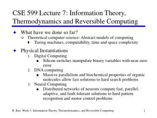
CSE 599 Lecture 7: Information Theory, Thermodynamics and Reversible Computing. What have we done so far? Theoretical computer science: Abstract models of computing Turing machines, computability, time and space complexity Physical Instantiations Digital Computing

E N D
CSE 599 Lecture 7: Information Theory, Thermodynamics and Reversible Computing • What have we done so far? • Theoretical computer science: Abstract models of computing • Turing machines, computability, time and space complexity • Physical Instantiations • Digital Computing • Silicon switches manipulate binary variables with near-zero error • DNA computing • Massive parallelism and biochemical properties of organic molecules allow fast solutions to hard search problems • Neural Computing • Distributed networks of neurons compute fast, parallel, adaptive, and fault-tolerant solutions to hard pattern recognition and motor control problems
Overview of Today’s Lecture • Information theory and Kolmogorov Complexity • What is information? • Definition based on probability theory • Error-correcting codes and compression • An algorithmic definition of information (Kolmogorov complexity) • Thermodynamics • The physics of computation • Relation to information theory • Energy requirements for computing • Reversible Computing • Computing without energy consumption? • Biological example • Reversibe logic gates Quantum computing (next week!)
Information and Algorithmic Complexity • 3 principal results: • Shannon’s source-coding theorem • The main theorem of information content • A measure of the number of bits needed to specify the expected outcome of an experiment • Shannon’s noisy-channel coding theorem • Describes how much information we can transmit over a channel • A strict bound on information transfer • Kolmogorov complexity • Measures the algorithmic information content of a string • An uncomputable function
What is information? • First try at a definition… • Suppose you have stored n different bookmarks on your web browser. • What is the minimum number of bits you need to store these as binary numbers? • Let I be the minimum number of bits needed. Then, 2I n I log2 n • So, the “information” contained in your collection of n bookmarks is I0 = log2 n
Deterministic information I0 • Consider a set of alternatives: X = {a1, a2, a3, …aK} • When the outcome is a3, we say x = a3 • I0(X) is the amount of information needed to specify the outcome of X • I0(X) = log2½X½ • We will assume base 2 from now on (unless stated otherwise) • Units are bits (binary digits) • Relationship between bits and binary digits • B = {0, 1} • X = BM = set of all binary strings of length M • I0(X) = log½BM½= log½2M½=M bits
Is this definition satisfactory? • Appeal to your intuition… • Which of these two messages contains more “information”? “Dog bites man” or “Man bites dog”
Is this definition satisfactory? • Appeal to your intuition… • Which of these two messages contains more “information”? “Dog bites man” or “Man bites dog” • Same number of bits to represent each message! • But, it seems like the second message contains a lot more information than the first. Why?
Enter probability theory… • Surprising events (unexpected messages) contain more information than ordinary or expected events • “Dog bites man” occurs much more frequently than “Man bites dog • Messages about less frequent events carry more information • So, information about an event varies inversely with the probability of that event • But, we also want information to be additive • If message xy contains sub-parts x and y, we want: • I(xy) = I(x) + I(y) • Use the logarithm function: log(xy) = log(x) + log(y)
New Definition of Information • Define the information contained in a message x in terms of log of the inverse probability of that message: • I(x) = log(1/P(x)) = - log P(x) • First defined rigorously and studied by Shannon (1948) • “A mathematical theory of communication” – electronic handout (PDF file) on class website. • Our previous definition is a special case: • Suppose you had n equally likely items (e.g. bookmarks) • For any item x, P(x) = 1/n • I(x) = log(1/P(x)) = log n • Same as before (minimum number of bits needed to store n items)
Review: Axioms of probability theory • Kolmogorov, 1933 • P(a) >= 0 where a is an event • P(l) = 1 where l is the certain event • P(a + b) = P(a) + P(b) where a and b are mutually exclusive • Kolmogorov (axiomatic) definition is computable • Probability theory forms the basis for information theory • Classical definition based on event frequencies (Bernoulli) is uncomputable:
Review: Results from probability theory • Joint probability of two events a and b: P(ab) • Independence • Events a and b are independent if P(ab) = P(a)P(b) • Conditional probability: P(a|b) = probability that event a happens given that b has happened • P(a|b) = P(ab)/P(b) • P(b|a) = P(ba)/P(a) = P(ab)/P(a) • We just proved Bayes’ Theorem: • P(a)is called the a priori probability of a • P(a½b) is called the a posteriori probability of a
Summary: Postulates of information theory 1. Information is defined in the context of a set of alternatives. The amount of information quantifies the number of bits needed to specify an outcome from the alternatives 2. The amount of information is independent of the semantics (only depends on probability) 3. Information is always positive 4. Information is measured on a logarithmic scale • Probabilities are multiplicative, but information is additive
In-Class Example • Message y contains duplicates: y = xx • Message x has probability P(x) • What is the information content of y? • Is I(y) = 2 I(x)?
In-Class Example • Message y contains duplicates: y = xx • Message x has probability P(x) • What is the information content of y? • Is I(y) = 2 I(x)? • I(y) = log(1/P(xx)) = log[1/(P(x|x)P(x))] = log(1/P(x|x)) + log(1/P(x)) = 0 + log(1/P(x)) = I(x) • Duplicates convey no additional information!
Definition: Entropy • The average self-information or entropy of an ensemble X= {a1, a2, a3, …aK} • E expected (or average) value
Properties of Entropy • 0 <= H(X) <= I0(X) • Equals I0(X) = log½X½ if all the ak’s are equally probable • Equals 0 if only one ak is possible • Consider the case where k = 2 • X = {a1, a2} • P(a1) = ; P(a2) = 1–
Examples • Entropy is a measure of randomness of the source producing the events • Example 1 : Coin toss: Heads or tails with equal probability • H = -(½ log ½ + ½ log ½) = -(½ (-1) + ½ (-1)) = 1 bit per coin toss • Example 2 : P(heads) = ¾ and P(tails) = ¼ • H = -(¾ log ¾ + ¼ log ¼) = 0.811 bits per coin toss • As things get less random, entropy decreases • Redundancy and regularity increases
Question • If we have N different symbols, we can encode them in log(N) bits. Example: English - 26 letters 5 bits • So, over many, many messages, the average cost/symbol is still 5 bits. • But, letters occur with very different probabilities! “A” and “E” much more common than “X” and “Q”. The log(N) estimate assumes equal probabilities. • Question: Can we encode symbols based on probabilities so that the average cost/symbol is minimized?
Shannon’s noiseless source-coding theorem • Also called the fundamental theorem. In words: • You can compress N independent, identically distributed (i.i.d.) random variables, each with entropy H, down to NH bits with negligible loss of information (as N) • If you compress them into fewer than NH bits you will dramatically lose information • The theorem: • Let X be an ensemble with H(X) = H bits. Let Hd(X) be the entropy of an encoding of X with allowable probability of error d • Given any > 0 and 0 < < 1, there exists a positive integer No such that, for N > No,
Comments on the theorem • What do the two inequalities tell us? • The number of bits that we need to specify outcomes x with vanishingly small error probability does not exceed H + • If we accept a vanishingly small error, the number of bits we need to specify x drops to N(H + ) • The number of bits that we need to specify outcomes x with large allowable error probability is at least H –
Source coding (data compression) • Question: How do we compress the outcomes XN? • With vanishingly small probability of error • How do we assign the elements of X such that the number of bits we need to encode XN drops to N(H + ) • Symbol coding: Given x = a3 a2 a7 … a5 • Generate codeword (x) = 01 1010 00 • Want Io((x)) ~ H(X) • Well-known coding examples • Zip, gzip, compress, etc. • The performance of these algorithms is, in general, poor when compared to the Shannon limit
Source-coding definitions • A code is a function : X B+ • B = {0, 1} • B+ the set of finite strings over B • B+ = {0, 1, 00, 01, 10, 11, 000, 001, …} • (x) = (x1) (x2) (x3) … (xN) • A code is uniquely decodable (UD) iff • : X+ B+ is one-to-one • A code is instantaneous iff • No codeword is the prefix of another • (x1) is not a prefix of (x2)
Huffman coding • Given X = {a1, a2, …aK}, with associated probabilities P(ak) • Given a code with codeword lengths n1, n2, …nk • The expected code length • No instantaneous, UD code can achieve a smaller than a Huffman code
Constructing a Huffman code • Feynman example: Encoding an alphabet • Code is instantaneous and UD: 00100001101010 = ANOTHER • Code achieves close to Shannon limit • H(X) = 2.06 bits; = 2.13 bits 1
Information channels • I(X;Y) is the average mutual information between X and Y • Definition: Channel capacity • The information capacity of a channel is: C = max[I(X;Y)] • The channel may add noise • Corrupting our symbols Input Output channel x y I(X;Y) what we know about X given Y H(X) entropy of input ensemble X
Example: Channel capacity Problem: A binary source sends equiprobable messages in a time T, using the alphabet {0, 1} with a symbol rate R. As a result of noise, a “0” may be mistaken for a “1”, and a “1” for a “0”, both with probability q. What is the channel capacity C? X Y Channel is discrete and memoryless
Example: Channel capacity (con’t) Assume no noise (no errors) T is the time to send the string, R is the rate The number of possible message strings is 2RT The maximum entropy of the source is Ho = log(2RT ) bits The source rate is (1/T) Ho = R bits per second The entropy of the noise (per transmitted bit) is Hn = qlog[1/q] + (1–q)log[1/(1–q)] The channel capacity C (bits/sec) = R – RHn = R(1 – Hn) C is always less than R (a fixed fraction of R)! We must add code bits to correct the received message
How many code bits must we add? • We want to send a message string of length M • We add codebits to M, thereby increasing its length to Mc • How are M, Mc, and q related? • M = Mc(1 – Hn) • Intuitively, from our example • Also see pgs. 106 – 110 of Feynman • Note: this is an asymptotic limit • May require a hugeMc
Shannon’s Channel-Coding Theorem • The Theorem: • There is a nonnegative channel capacity C associated with each discrete memoryless channel with the following property: For any symbol rate R < C, and any error rate > 0, there is a protocol that achieves a rate >= R and a probability of error <= • In words: • If the entropy of our symbol stream is equal to or less than the channel capacity, then there exists a coding technique that enables transmission over the channel with arbitrarily small error • Can transmit information at a rate H(X) <= C • Shannon’s theorem tells us the asymptotically maximum rate • It does not tell us the code that we must use to obtain this rate • Achieving a high rate may require a prohibitively long code
Error-correction codes • Error-correcting codes allow us to detect and correct errors in symbol streams • Used in all signal communications (digital phones, etc) • Used in quantum computing to ameliorate effects of decoherence • Many techniques and algorithms • Block codes • Hamming codes • BCH codes • Reed-Solomon codes • Turbo codes
Hamming codes • An example: Construct a code that corrects a single error • We add m check bits to our message • Can encode at most (2m – 1) error positions • Errors can occur in the message bits and/or in the check bits • If n is the length of the original message then 2m – 1 >= (n + m) • Examples: • If n = 11, m = 4: 24 – 1= 15 >= (n + m) = 15 • If n = 1013, m = 10: 210 – 1= 1023 >= (n + m) = 1023
Hamming codes (cont.) • Example: An 11/15 SEC Hamming code • Idea: Calculate parity over subsets of input bits • Four subsets: Four parity bits • Check bit x stores parity of input bit positions whose binary representation holds a “1” in position x: • Check bit c1: Bits 1,3,5,7,9,11,13,15 • Check bit c2: Bits 2,3,6,7,10,11,14,15 • Check bit c3: Bits 4,5,6,7,12,13,14,15 • Check bit c4: Bits 8,9,10,11,12,13,14,15 • The parity-check bits are called a syndrome • The syndrome tells us the location of the error Position in message binary decimal 0001 1 0010 2 0011 3 0100 4 0101 5 0110 6 0111 7 1000 8 1001 9 1010 10 1011 11 1100 12 1101 13 1110 14 1111 15
Hamming codes (con’t) • The check bits specify the error location • Suppose check bits turn out to be as follows: • Check c1 = 1 (Bits 1,3,5,7,9,11,13,15) • Error is in one of bits 1,3,5,7,9,11,13,15 • Check c2 = 1 (Bits 2,3,6,7,10,11,14,15) • Error is in one of bits 3,7,11,15 • Check c3 = 0 (Bits 4,5,6,7,12,13,14,15) • Error is in one of bits 3,11 • Check c4 = 0 (Bits 8,9,10,11,12,13,14,15) • So error is in bit 3!!
Hamming codes (cont.) • Example: Encode 10111011011 • Code position: 15 14 13 12 11 10 9 8 7 6 5 4 3 2 1 • Code symbol: 1 0 1 1 1 0 1 c4 1 0 1 c3 1 c2 c1 • Codeword: 1 0 1 1 1 0 1 1 1 0 1 1 1 0 1 • Notice that we can generate the code bits on the fly! • What if we receive 101100111011101? • c4 = 1 101100111011101 • c3 = 0 101100111011101 • c2 = 1 101100111011101 • c1 = 1 101100111011101 • The error is in location 1011 = 1110
Kolmogorov Complexity (Algorithmic Information) • Computers represent information as stored symbols • Not probabilistic n the Shannon sense) • Can we quantify information from an algorithmic standpoint? • Kolmogorov complexity K(s) of a finite binary string s is the single, natural number representing the minimum length (in bits) of a program p that generates s when run on a Universal Turing machine U • K(s) is the algorithmic information content of s • Quantifies the “algorithmic randomness” of the string • K(s) is an uncomputable function • Similar argument to the halting problem • How do we know when we have the shortest program?
Kolmogorov Complexity: Example • Randomness of a string defined by shortest algorithm that can print it out. • Suppose you were given the binary string x: “11111111111111….11111111111111111111111” (1000 1’s) • Instead of 1000 bits, you can compress this string to a few tens of bits, representing the length |P| of the program: • For I = 1 to 1000 • Print “1” • So, K(x) <= |P| • Possible project topic: Quantum Kolmogorov complexity?
5-minute break… Next: Thermodynamics and Reversible Computing
Thermodynamics and the Physics of Computation • Physics imposes fundamental limitations on computing • Computers are physical machines • Computers manipulate physical quantities • Physical quantities represent information • The limitations are both technological and theoretical • Physical limitations on what we can build • Example: Silicon-technology scaling • Major limiting factor in the future: Power Consumption • Theoretical limitations of energy consumed during computation • Thermodynamics and computation
Principal Questions of Interest • How much energy must we use to carry out a computation? • The theoretical, minimum energy • Is there a minimum energy for a certain rate of computation? • A relationship between computing speed and energy consumption • What is the link between energy and information? • Between information–entropy and thermodynamic–entropy • Is there a physical definition for information content? • The information content of a message in physical units
Main Results • Computation has no inherent thermodynamic cost • A reversible computation, that proceeds at an infinitesimal rate, consumes no energy • Destroying information requires kTln2 joules per bit • Information-theoretic bits (not binary digits) • Driving a computation forward requires kTln(r) joules per step • r is the rate of going forward rather than backward
Basic thermodynamics • First law: Conservation of energy • (heat put into system) + (work done on system) = increase in energy of a system • DQ + DW = DU • Total energy of the universe is constant • Second law: It is not possible to have heat flow from a colder region to a hotter region i.e. DQ/T >= 0 • Change in Entropy DS = DQ/T • Equality holds only for reversible processes • The entropy of the universe is always increasing
Heat engines • A basic heat engine: Q2 = Q1 – W • T1 and T2 are temperatures • T1 > T2 • Reversible heat engines are those that have: • No friction • Infinitesimal heat gradients • The Carnot cycle: Motivation was steam engine • Reversible • Pumps heat DQ from T1 to T2 • Does work W = DQ
The Second Law • No engine that takes heat Q1 at T1 and delivers heat Q2 at T2 can do more work than a reversible engine • W = Q1 – Q2 = Q1(T1 – T2) / T1 • Heat will not, by itself, flow from a cold object to a hot object
Thermodynamic entropy • If we add heat Q reversibly to a system at fixed temperature T, the increase in entropy of the system is S = Q/T • S is a measure of degrees of freedom • The probability of a configuration • The probability of a point in phase space • In a reversible system, the total entropy is constant • In an irreversible system, the total entropy always increases
Thermodynamic versus Information Entropy • Assume a gas containing N atoms • Occupies a volume V1 • Ideal gas: No attraction or repulsion between particles • Now shrink the volume • Isothermally (at constant temperature, immerse in a bath) • Reversibly, with no friction • How much work does this require?
Compressing the gas • From mechanics • work = force × distance • force = pressure × (area of piston) • volume change = (area of piston) × distance • Solving: • From gas theory • The idea gas law: • N number of molecules • k Boltzmann’s constant (in joules/Kelvin) • Solving:
A few notes • W is negative because we are doing work on the gas:V2 < V1 • W would be positive if the gas did work for us • Where did the work go? • Isothermal compression • The temperature is constant (same before and after) • First law: The work went into heating the bath • Second law: We decreased the entropy of the gas and increased the entropy of the bath
Free energy and entropy • The total energy of the gas, U, remains unchanged • Same number of particles • Same temperature • The “free energy” Fe, and the entropy S both change • Both are related to the number of states (degrees of freedom) • Fe = U – TS • For our experiment, change in free energy is equal to the work done on the gas and U remains unchanged DFe is the (negative) heat siphoned off into the bath
Special Case: N = 1 • Imagine that our gas contains only one molecule • Take statistical averages of same molecule over time rather than over a population of particles • Halve the volume • Fe increases by +kTln2 • S decreases by kln2 • But U is constant • What’s going on? • Our knowledge of the possible locations of the particle has changed! • Fewer places that themolecule can be in, now that volume has been halved • The entropy, a measure of the uncertainty of a configuration, has decreased