Download
1 / 91
980 likes | 1.26k Views
The Transit Method. Photometric Spectroscopic (next time). Detection and Properties of Planetary Systems 18 Apr: Introduction and Background: 25 Apr: The Radial Velocity Method 02 May: Results from Radial Velocity Searches 09 May: Astrometry 16 May: The Transit Method

E N D
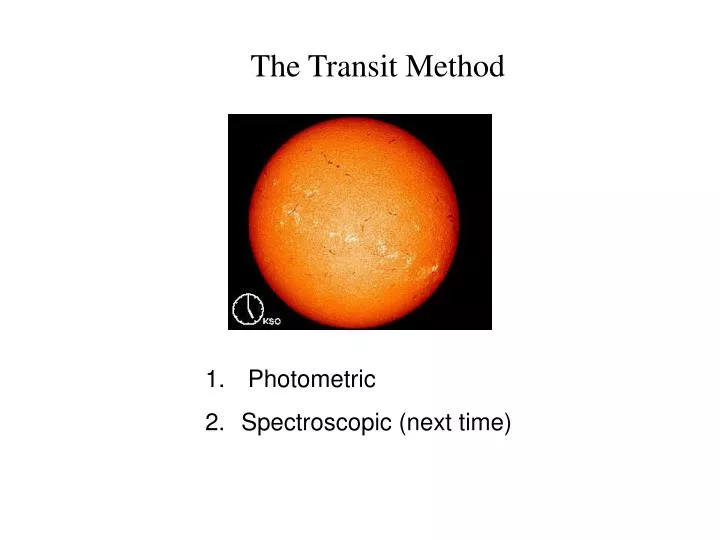
The Transit Method • Photometric • Spectroscopic (next time)
Detection and Properties of Planetary Systems 18 Apr: Introduction and Background: 25 Apr: The Radial Velocity Method 02 May: Results from Radial Velocity Searches 09 May: Astrometry 16 May: The Transit Method 23 May: Planets in other Environments (Eike Guenther) 30 May: Transit Results: Ground-based 06 Jun: Transit Results: Space-based 13 Jun: Exoplanet Atmospheres 20 Jun: Direct Imaging 27 Jun: Microlensing 04 Jul: No Class 11 Jul: Planets in Extreme Environments: Planets around evolved stars 18 Jul: Habitable Planets: Where are the other Earths?
Literature • Contents: • Our Solar System from Afar (overview of detection methods) • Exoplanet discoveries by the transit method • What the transit light curve tells us • The Exoplanet population • Transmission spectroscopy and the Rossiter-McLaughlin effect • Host Stars • Secondary Eclipses and phase variations • Transit timing variations and orbital dynamics • Brave new worlds By Carole Haswell
Historical Context of Transiting Planets (Venus) Transits (in this case Venus) have played an important role in the history of research of our solar system. Kepler‘s law could give us the relative distance of the planets from the sun in astronomical units, but one had to determine the AU in order to get absolute distances. This could be done by observing Venus transits from two different places on the Earth and using triangulation. This would fix the distance between the Earth and Venus.
Historical Context of Transiting Planets (Venus) From wikipedia Jeremiah Horrocks was the first to attempt to observe a transit of Venus. Kepler predicted a transit in 1631, but Horrocks re-calculated the date as 1639. Made a good guess as to the size of Venus and estimated the Astronomical Unit to be 0.64 AU, smaller than the current value but better than the value at the time.
Transits of Venus occur in pairs separated by 8 years and these were the first international efforts to measure these events. Le Gentil‘s observatory One of these expeditions was by Guilaume Le Gentil who set out to the French colony of Pondicherry in India to observe the 1761 transit. He set out in March and reached Mauritius (Ile de France) in July 1760. But war broke out between France and England so he decided to take a ship to the Coromandel Coast. Before arriving the ship learned that the English had taken Pondicherry and the ship had to return to Ile de France. The sky was clear but he could not make measurements due to the motion of the ship. Coming this far he decided to just wait for the next transit in 8 years. He then mapped the eastern coast of Madagascar and decided to observe the second transit from Manilla in the Philippines. The Spanish authorities there were hostile so he decided to return to Pondicherry where he built an observatory and patiently waited. The month before was entirely clear, but the day of the transit was cloudy – Le Gentil saw nothing. This misfortune almost drove him crazy, but he recovered enough to return to France. The return trip was delayed by dysentry, the ship was caught in a storm and he was dropped off on the Ile de Bourbon where he waited for another ship. He returned to Paris in 1771 eleven years after he started only to find that he had been declared dead, been replaced in the Royal Academy of Sciences, his wife had remarried, and his relatives plundered his estate. The king finally intervened and he regained his academy seat, remarried, and lived happily for another 21 years.
Historical Context of Transiting Planets (Venus) From wikipedia Mikhail Lomonosov predicted the existence of an atmosphere on Venus from his observations of the transit. Lomonosov detected the refraction of solar rays while observing the transit and inferred that only refraction through an atmosphere could explain the appearance of a light ring around the part of Venus that had not yet come into contact with the Sun's disk during the initial phase of transit.
On 6. June 2012 the second transit of the 8-year pairs takes place. Venus transit im June 2012!
Venus limb solar
R* DI What are Transits and why are they important? The drop in intensity is give by the ratio of the cross-section areas: DI = (Rp /R*)2 = (0.1Rsun/1 Rsun)2 = 0.01 for Jupiter Radial Velocity measurements => Mp (we know sin i !) => density of planet → Transits allows us to measure the physical properties of the planets
What can we learn about Planetary Transits? The radius of the planet The orbital inclination and the mass when combined with radial velocity measurements Density → first hints of structure The Albedo from reflected light The temperature from radiated light Atmospheric spectral features In other words, we can begin to characterize exoplanets
Comparison of the Giant Planets 1.24 0.62 1.25 1.6 Mean density (gm/cm3) http://www.freewebs.com/mdreyes3/chaptersix.htm
10 Iron enriched Earth-like 7 Earth Mercury r (gm/cm3) No iron 5 Venus Mars 4 3 Moon The radius, mass, and density are the first clues about the internal structure 2 From Diana Valencia 1 2 1.8 0.4 0.2 1 0.6 0.8 1.2 1.4 1.6 Radius (REarth)
Earth Venus Earth and Venus have a core that is ~80% iron extending out to a radius of 0.3 to 0.5 of the planet
Moon Mercury • Crust: 100 km • Silicate Mantle (25%) • Nickel-Iron Core (75%) Mercury has a very large iron core and thus a high density for its small size The moon has a very small core, but a large mantle (≈70%)
90+q Porb = 2p sin i di / 4p = 90-q Transit Probability i = 90o+q q R* a sin q = R*/a = |cos i| a is orbital semi-major axis, and i is the orbital inclination1 –0.5 cos (90+q) + 0.5 cos(90–q) = sin q = R*/a for small angles 1by definition i = 90 deg is looking in the orbital plane
2R* P (4p2)1/3 t 2p P2/3 M*1/3G1/3 Transit Duration t = 2(R* +Rp)/v where v is the orbital velocity and i = 90 (transit across disk center) For circular orbits v = 2pa/P From Keplers Law’s: a = (P2 M*G/4p2)1/3 t1.82 P1/3 R* /M*1/3 (hours) In solar units, P in days Note t3 ~ (rmean)–1 i.e. it is related to the mean density of the star
Transit Duration Note: The transit duration gives you an estimate of the stellar radius 0.55 t M1/3 Rstar = P1/3 Most Stars have masses of 0.1 – 4 solar masses. M⅓ = 0.46 – 1.6 R in solar radii M in solar masses P in days t in hours
For more accurate times need to take into account the orbital inclination for i 90o need to replace R* with R: R2 + d2cos2i = R*2 R = (R*2– d2 cos2i)1/2 d cos i R* R
Making contact: Note: for grazing transits there is no 2nd and 3rd contact • First contact with star • Planet fully on star • Planet starts to exit • Last contact with star 1 4 2 3
N is the number of stars you would have to observe to see a transit, if all stars had such a planet. This is for our solar system observed from a distant star.
Note the closer a planet is to the star: • The more likely that you have a favorable orbit for a transit • The shorter the transit duration • Higher frequency of transits → The transit method is best suited for short period planets. Prior to 51 Peg it was not really considered a viable detection method.
Shape of Transit Curves 2 tflat [R*– Rp]2– d2 cos2i tflat = ttotal [R*+ Rp]2– d2 cos2i ttotal Note that when i = 90o tflat/ttotal = (R*– Rp)/( R* + Rp)
Shape of Transit Curves HST light curve of HD 209458b A real transit light curve is not flat
Temperature profile of photosphere Bottom of photosphere 10000 8000 z Temperature 6000 4000 q2 z=0 q1 dz tn =1 surface Top of photosphere Shape of Transit Curves Effects of Limb Darkening (or why the curve is not flat). z increases going into the star
To probe limb darkening in other stars.. ..you can use transiting planets No limb darkening transit shape At the limb the star has less flux than is expected, thus the planet blocks less light
Report that the transit duration is increasing with time, i.e. the inclination is changing: However, Kepler shows no change in the inclination!
To model the transit light curve and derive the true radius of the planet you have to have an accurate limb darkening law. Problem: Limb darkening is only known very well for one star – the Sun!
Why Worry about Limb Darkening? Suppose someone observes a transit in the optical. The „diameter“ of the stellar disk is determined by the limb darkening Years later you observe the transit at 10000 Ang. The star has less limb darkening, it thus has a larger „apparent diameter. You calculate a longer duration transit because you do not take into account the different limb darkening
And your wrong conclusion: More limb darkening → short transit duration Less limb darkening in red → longer transit duration → orbital inclination has changed!
Shape of Transit Curves Grazing eclipses/transits These produce a „V-shaped“ transit curve that are more shallow Planet hunters like to see a flat part on the bottom of the transit
Probability of detecting a transit Ptran: Ptran= Porbx fplanetsx fstars x DT/P Porb = probability that orbit has correct orientation fplanets = fraction of stars with planets fstars = fraction of suitable stars (Spectral Type later than F5) DT/P = fraction of orbital period spent in transit
Estimating the Parameters for 51 Peg systems Porb Period ≈ 4 days → a = 0.05 AU =10 Rסּ Porb 0.1 fplanets Although the fraction of giant planet hosting stars is 5-10%, the fraction of short period planets is smaller, or about 0.5–1%
Estimating the Parameters for 51 Peg systems fstars This depends on where you look (galactic plane, clusters, etc.) but typically about 30-40% of the stars in the field will have radii (spectral type) suitable for transit searches.
Radius as a function of Spectral Type for Main Sequence Stars A planet has a maximum radius ~ 0.15 Rsun. This means that a star can have a maximum radius of 1.5 Rsun to produce a transit depth consistent with a planet → one must know the type of star you are observing!
Take 1% as the limiting depth that you can detect a transit from the ground and assume you have a planet with 1 RJ = 0.1 Rsun Example: B8 Star: R=3.8 RSun DI = (0.1/3.8)2 = 0.0007 Suppose you detect a transit event with a depth of 0.01. This corresponds to a radius of 50 RJupiter = 0.5 Rsun Additional problem: It is difficult to get radial velocity confirmation on transits around early-type stars Transit searches on Early type, hot stars are not effective
You also have to worry about late-type giant stars Example: A K III Star can have R ~ 10 RSun DI = 0.01 = (Rp/10)2 → Rp = 1 RSun! Unfortunately, background giant stars are everywhere. In the CoRoT fields, 25% of the stars are giant stars Giant stars are relatively few, but they are bright and can be seen to large distances. In a brightness limited sample you will see many distant giant stars.
Along the Main Sequence Spectral Type Spectral Type DI/I Stellar Mass (Msun) Stellar Mass (Msun) The photometric transit depth for a 1 RJup planet
Along the Main Sequence Planet Radius (RJup) 1 REarth Stellar Mass (Msun) Assuming a 1% photometric precision this is the minimum planet radius as a function of stellar radius (spectral type) that can be detected
Estimating the Parameters for 51 Peg systems Fraction of the time in transit Porbit≈ 4 days Transit duration ≈ 3 hours DT/P 0.08 Thus the probability of detecting a transit of a planet in a single night is 0.00004.
For each test orbital period you have to observe enough to get the probability that you would have observed the transit (Pvis) close to unity.
E.g. a field of 10.000 Stars the number of expected transits is: Ntransits = (10.000)(0.1)(0.01)(0.3) = 3 Probability of right orbit inclination Frequency of Hot Jupiters Fraction of stars with suitable radii So roughly 1 out of 3000 stars will show a transit event due to a planet. And that is if you have full phasecoverage! CoRoT: looks at 10,000-12,000 stars per field and is finding on average 3 Hot Jupiters per field. Similar results for Kepler Note: Ground-based transit searches are finding hot Jupiters 1 out of 30,000 – 50,000 stars → less efficient than space-based searches
Catching a transiting planet is thus like playing Lotto. To win in LOTTO you have to • Buy lots of tickets → Look at lots of stars • Play often → observe as often as you can The obvious method is to use CCD photometry (two dimensional detectors) that cover a large field. You simultaneously record the image of thousands of stars and measure the light variations in each.
Confirming Transit Candidates A transit candidate found by photometry is only a candidate until confirmed by spectroscopic measurement (radial velocity) Any 10–30 cm telescope can find transits. To confirm these requires a 2–10 m diameter telescope with a high resolution spectrograph. This is the bottleneck. Current programs are finding transit candidates faster than they can be confirmed.
Light curve for HD 209458 Transit Curve: 10 cm telescope
Radial Velocity Curve for HD 209458 Transit phase = 0 Period = 3.5 days Msini = 0.63 MJup Radial Velocity Curve: 2-10 m telescopes