V15 – protein docking, FFT, electron tomography

1. V15 – protein docking, FFT, electron tomography Fast Fourier Transform Electron Tomography Bioinformatics III

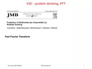
2. Prediction of Assemblies from Pairwise Docking CombDock: first fully automated approach for predicting hetero multimolecular assembly only based on structural models of its protein subunits. Problem appears more difficult than the pairwise docking problem; it is NP-hard. Idea: exploit additional geometric constraints embraced in the combinatorial problem. Input: a set of protein structural models. Unlike a 3D puzzle, where two connected pieces in the puzzle solution match perfectly, we would like to tolerate some extent of penetration, due to the flexible nature of the proteins. Inbar et al., J. Mol. Biol. 349, 435 (2005) Bioinformatics III

3. Pairwise docking: Katchalski-Kazir algorithm; FTDOCK Discretize proteins A and B on a grid. Every node is assigned a value Use FFT to compute correlation efficiently. Output: solutions with best surface complementarity. Gabb et al. J. Mol. Biol. (1997) Bioinformatics III

4. (1) All pairs docking module Module gets as its input N protein structures  predict pairwise interactions. Perform pairwise docking for each of the N (N - 1) / 2 pairs of proteins. Keep K best solutions for each pair of proteins. Since pairwise-docking is a difficult problem, the correct solution may be among the first few hundred solutions.  K should be set reasonably high. Here, K was varied from dozens to hundreds. Inbar et al., J. Mol. Biol. 349, 435 (2005) Bioinformatics III

5. (2) Combinatorial assembly module Input: N subunits and N (N - 1) / 2 sets of K scored transformations. These are the candidate interactions. Reduction to a spanning tree Build weighted graph representing the input: each structural unit = vertex each transformation = edge connecting the corresponding vertices edge weight = score of the transformation  Since the input contains K transformations for each pair of subunits, we have a complete graph with K parallel edges between each pair of vertices. Inbar et al., J. Mol. Biol. 349, 435 (2005) Bioinformatics III

6. (2) Combinatorial assembly module For two subunits, each candidate complex is represented by an edge and the two vertices. In the case of N structural units a candidate complex is represented by a spanning tree = a subgraph of the input graph that connects all vertices and has no circles. Each spanning tree of the input graph represents a complex of all the input structural units. The problem of finding complexes is equivalent to finding spanning trees. The number of spanning trees in a complete graph with no parallel edges is NN-2 (Cayley‘s formula). Since the input graph has K parallel edges between each pair of vertices, the number of spanning trees is NN-2 KN-1 .  Exhaustive searches are infeasible. Inbar et al., J. Mol. Biol. 349, 435 (2005) Bioinformatics III

7. (2) Combinatorial assembly module:algorithm Algorithm uses 2 basic principles: (1) hierarchical construction of the spanning tree (2) greedy selection of subtrees Different trees share common trees  generate trees with n vertices by connecting two trees of smaller size (that were previously generated) with an input edge. Thus, the common parts of different trees are generated only once. When connecting subtrees, validate only the inter-subtree constraints.  need to check whether there are severe penetrations in the complex only between pairs of subunits, where each is represented by a different subtree. Inbar et al., J. Mol. Biol. 349, 435 (2005) Bioinformatics III

8. (2) Combinatorial assembly module:algorithm Stage 1: algorithm constructs trees of size 1. Each tree contains a single vertex that represents a subunit. Stage i: the tree complexes that consist of exactly i vertices (subunits) are generated by connecting two trees generated at a lower stage with an input edge transformation. Tree complexes that fulfil the penetration constraint are kept for the next stages. Because it is impractical to search all valid spanning trees, the algorithm performs a greedy selection of subtrees. For each subset of vertices, the algorithm keeps only the D best-scoring valid trees that connect them. The tree score is the sum of its edge weights. Inbar et al., J. Mol. Biol. 349, 435 (2005) Bioinformatics III

9. Flowchart www.cs.tau.ac.il/~inbaryuv/combdoc/ Bioinformatics III

10. Example The construction of the third-best scoring solution of arp2/3 complex (RMSD 1.2 Å ). The combinatorial assembly algorithm is hierarchical: at the first stage, each complex consists of a single subunit. At the ith stage it constructs complexes that consist of i subunits by connecting complexes of smaller size using one of the input candidate transformations. The arp2/3 complex consists of seven subunits shown at the top. In this Figure we present only the complexes of the different stages that are relevant to the construction of the third-best scoring solution (at the bottom of the Figure). Along with each complex is its corresponding subgraph, where the vertices represent the subunits and the edges represent the pairwise interactions that were used to construct the complex. In each graph, the red edge represents the transformation of the current stage, while blue edges represent transformations of previous stages. Inbar et al., J. Mol. Biol. 349, 435 (2005) Bioinformatics III

11. Final scoring The geometric score evaluates the shape complementarity between the subunits: check distances between surface points on adjacent subunits. Close surface points increase score, penetrating surface points decrease score. Physico-chemical component of the final score counts the #surface points that belong to non-polar atoms = gives an estimate of the hydrophobic effect. Clustering of solutions: (1) compute contact maps between subunits: array of N ( N – 1 ) bins. If two subunits are in contact within the complex, set the corresponding bit to 1, and to 0 otherwise. (2) superimpose complexes that have the same contact map and compute RMSD between C atoms. If this distance is less than a threshold, consider complexes as members of a cluster. For each cluster, keep only the complex with the highest score. Inbar et al., J. Mol. Biol. 349, 435 (2005) Bioinformatics III

12. Performance for known complexes Inbar et al., J. Mol. Biol. 349, 435 (2005) Bioinformatics III

13. Method works with different contact topologies. The near-native solutions for two complexes with different contact topologies. Left: CombDock solution, Right: solution superposed on the crystal structure (gray thiner lines). (a) the sixth-best scoring solution for the IkBa/NF-kB complex of an unbound input, RMSD 1.9 Å. The p65 subunit was extracted from a homodimer structure (PDB 1BFT). The structure used for the IkBa subunit was generated by MODELLER6 v2 using bcl-3 (PDB 1k1b) as the template structure; (b) the second-best scoring solution of VHL/elonginC/elonginB complex (PDB 1vcb), with an RMSD of 0.5 Å . Each complex consists of three subunits but, while in the IkBa/NF-kB complex all the subunits are in contact with each other, in the VHL/elonginC/ elonginB complex the elonginC is the core of the complex (in yellow) and VHL (in blue) and elonginB (in red) are not in contact. The algorithm was able to predict a near-native solution for both complexes regardless of their contact topologies. Inbar et al., J. Mol. Biol. 349, 435 (2005) Bioinformatics III

14. Examples of large complexes Left: CombDock solution, Right: solution superposed on the crystal structure (gray thinner lines). The solutions are: (a) the third-best scoring assembly of the seven subunits of the arp2/3 complex, RMSD 1.2 Å ; (b) the bestranked complex of the ten subunits of RNA polymerase II, RMSD 1.4 Å. Inbar et al., J. Mol. Biol. 349, 435 (2005) Bioinformatics III

15. Discussion of CombDock For the five different targets, CombDock predicted at least one near-native solution and ranked it in the top ten for both bound and unbound cases. Problem in evaluating performance: full sets of „unbound“ structures are not available for complexes with a higher number of subunits. It is unlikely that this version of the algorithm (using rigid protein conformations) will be able to correctly assemble such complexes if the input subunits involve significant conformational changes.  future version should include hinge-bending movements of protein subunits. Inbar et al., J. Mol. Biol. 349, 435 (2005) Bioinformatics III

16. Fast Fourier Transform Discrete Fourier Transform of a function from a finite number of its sampled points. Suppose that we have N consecutive sampled values so that the sampling interval is . Let us assume that N is even. The discrete Fourier transform of the N points hk is The formula for the discrete inverse Fourier transform, which recovers the set of hk‘sexactly from the Hn‘s is: after: Numerical Recipes Bioinformatics III

17. Fast Fourier Transform How much computation is involved in computing the discrete Fourier transform of N points? Until the mid-1960s, the standard answer was this: Define W as the complex number Then we can write The vector of hk‘s is multiplied by a matrix whose (n,k)th element is the constant W to the power n  k. The matrix multiplication produces a vector result whose components are the Hn’s. This matrix multiplication requires N2complex multiplications, plus a smaller number of operations to generate the required powers of W. So, the discrete Fourier transform appears to be an O(N2) process. Bioinformatics III

18. Fast Fourier Transform However, the discrete Fourier transform (in 1 dimension) can be computed in O(N log2 N) operations by an algorithm called the Fast Fourier Transform. With N = 106, the difference between O(N2) and O(N log2 N) is 30 CPU seconds against 2 CPU weeks! The FFT algorithm became generally known in the mid-1960s from the work of J.W. Cooley and J.W. Tukey. In fact, efficient methods to compute discrete Fourier transforms had been independently discovered many times, starting with Gauss in 1805. Bioinformatics III

19. FFT by Danielson and Lanczos (1942) D. and L. showed that a discrete Fourier transform of length N can be rewritten as the sum of two discrete Fourier transforms, each of length N/2. One of the two is formed from the even-numbered points of the original N, the other from the odd-numbered points. W is the same constant as before. Fke : k-th component of the Fourier transform of length N/2 formed from the even components of the original fj’s Fko : k-th component of the Fourier transform of length N/2 formed from the odd components of the original fj ’s Bioinformatics III

20. FFT by Danielson and Lanczos (1942) The wonderful property of the Danielson-Lanczos-Lemma is that it can be used recursively. Having reduced the problem of computing Fk to that of computing Fke and Fko , we can do the same reduction of Fke to the problem of computing the transform of its N/4 even-numbered input data and N/4 odd-numbered data. We can continue applying the DL-Lemma until we have subdivided the data all the way down to transforms of length 1. What is the Fourier transform of length one? It is just the identity operation that copies its one input number into its one output slot. For every pattern of log2Ne‘s and o‘s, there is a one-point transform that is just one of the input numbers fn Bioinformatics III

21. FFT by Danielson and Lanczos (1942) The next trick is to figure out which value of n corresponds to which pattern of e‘s and o‘s in Answer: reverse the pattern of e‘s and o‘s, then let e = 0 and o = 1, and you will have, in binary the value of n. Idea: this works because the successive subdividisions of the data into even and odd are tests of successive low-order (least significant) bits of n. This idea of bit reversal can be exploited in a very clever way which, along with the DL-Lemma, makes FFT practical: Suppose we take the original vector of data fjand rearrange it into bit-reversed order, so that the individual numbers are in the order not of j, but of the number obtained by bit-reversing j. Bioinformatics III

22. FFT by Danielson and Lanczos (1942) Reordering an array (here of length 8) by bit reversal, (a) between two arrays, versus (b) in place. The points as given are the one-point transforms. We combine adjacent pairs to get two-point transforms, then combine adjacent pairs of pairs to get 4-point transforms, and so on until the first and second halves of the whole data set are combined into the final transform. Each combination takes of order N operations, and there are log2N combinations. This, then, is the structure of an FFT algorithm. Bioinformatics III

23. New challenge: Electron Tomography Method overview a) The electron beam of an EM microscope is scattered by the central object and the scattered electrons are detected on the black plate. By tilting the object in small steps, collect electrons scattered at different angles. b) reconstruction in the computer. Back-projection (Fourier method) of the scatter-information at different angles. The superposition generates a three-dimensional tomogrom. Sali et al. Nature 422, 216 (2003) Bioinformatics III

24. Identification of macromolecular complexes in cryoelectron tomograms of phantom cells Idea: construct model system with well-defined properties. Prepare „phantom cells“ (ca. 400 nm diameter) with well-defined contents: liposomes filled with thermosomes and 20S proteasomes. Thermosome: 933 kD, 16 nm diameter, 15 nm height, subunits assemble into toroidal structure with 8-fold symmetry. 20S proteasome: 721 kD, 11.5 nm diameter, 15 nm height, subunits assemble into toroidal structure with 7-fold symmetry. Collect Cryo-EM pictures of phantom cells for a tilt series from -70º until +70º with 1.5º increments. Aim: identify and map the 2 types of proteins in the phantom cell. This is a problem of matching a template, ideally derived from a high-resolution structure, to an image feature, the target structure. Frangakis et al., PNAS 99, 14153 (2002) Bioinformatics III

25. Detection and idenfication strategy The correlation of two functions is defined as Correlation theorem for the transform pairs: Frangakis et al., PNAS 99, 14153 (2002) Bioinformatics III

26. Search strategy • Adjust pixel size of templates to the pixel size of the EM 3D reconstruction. • The gray value of a voxel (volume element) containing ca. 30 atoms is obtained by summation of the atomic number of all atoms positioned in it. • Possible search strategies: • Scan reconstructed volume by using small boxes of the size of the target structure (real space method) • Paste template into a box of the size of the reconstructed volume (Fourier space method). This method is much more efficient. Frangakis et al., PNAS 99, 14153 (2002) Bioinformatics III

27. Correlation with Nonlinear Weighting The correlation coefficient CC is a measure of similarity of two features e.g. a signal x (image)and a template r both with the same size R. Expressed in one dimension: are the mean values of the subimage and the template. The denominators are the variances To derive the local-normalized cross correlation function or, equivalently, the correlation coefficients in a defined region R around each voxel k, which belongs to a large volume N (whereby N >> R), nonlinear filtering has to be applied. This filtering is done in the form of nonlinear weighting. Frangakis et al., PNAS 99, 14153 (2002) Bioinformatics III

28. Raw data • Central x-y slices through the 3D reconstructions of ice-embedded phantom cells filled with • 20S proteasomes, • thermosomes, • and a mixture of both particles. • At low magnification, the macromolecules appear as small dots. Frangakis et al., PNAS 99, 14153 (2002) Bioinformatics III

29. Correlation coefficients • Histogram of the correlation coefficients of the particles found in the proteasome-containing phantom cell scanned with the "correct" proteasome and the "false" thermosome template. Of the 104 detected particles, 100 were identified correctly. The most probable correlation coefficient is 0.21 for the proteasome template and 0.12 for the thermosome template. • Histogram of the correlation coefficients of the particles found in the thermosome-containing phantom cell. Of the 88 detected particles, 77 were identified correctly. The most probable correlation value is 0.21 for the thermosome template and 0.16 for the proteasome template. • Detection in (a) works well, but is somehow problematic in (b) because (correct) thermosome and proteasome are not well separated. Frangakis et al., PNAS 99, 14153 (2002) Bioinformatics III

30. Reconstruction of phantom cell Volume-rendered representation of a reconstructed ice-embedded phantom cell containing a mixture of thermosomes and 20S proteasomes. After applying the template-matching algorithm, the protein species were identified according to the maximal correlation coefficient. The molecules are represented by their averages; thermosomes are shown in blue, the 20S proteasomes in yellow. The phantom cell contained a 1:1 ratio of both proteins. The algorithm identifies 52% as thermosomes and 48% as 20S proteasomes. Frangakis et al., PNAS 99, 14153 (2002) Bioinformatics III

31. Electron tomography • Method has very high computational cost. • Observation: biological cells are not packed so densely as expected, • allowing the identification of single proteins and protein complexes • Problem for real cells: molecular crowding. • Potential difficulties to identify spots. • - need to increase spatial resolution of tomograms Frangakis et al., PNAS 99, 14153 (2002) Bioinformatics III

32. Reconstruction of endoplasmatic reticulum Picture rights shows rough endoplasmatic reticulum (membrane network in eukaryotic cells that generates proteins and new membranes) coated with ribosomes. The picture is taken from an intact cell. Membranes are shown in blue, the ribosomes in green-yellow. http://science.orf.at/science/news/61666 Dept. of Structural Biology, Martinsried Bioinformatics III

33. Reconstruction of the Golgi apparatus The Golgi complex is the organelle in which newly synthesized lipids and proteins are modified and targeted for distribution to various cellular and extracellular destinations. HVEM tomographic reconstruction of a portion of the Golgi ribbon from a fast frozen, freeze-substitution fixed NRK cell. Two serial 4-nm slices extracted from the tomogram are shown in a and b. Comparison of the images shows how little is changed from one such slice to its neighbor; e.g., the position of the microtubule (red arrow). (a) Membranes of individual Golgi and ER cisternae are clearly seen. (b) In analyzing the data, different cisternae were modeled by placing points along the membranes that delimit them, connecting the points with colored line segments, and building closed contours that model the different membrane compartments of a given slice. Ladinsky et al. J. Cell. Biol. 144, 1135 (1999) Bioinformatics III

34. Reconstruction of the Golgi apparatus c and d are renditions of the surfaces fit to all of the contours for each object modeled in this Golgi region. The model viewed in c is in the same orientation as the tomographic slices. d shows a cisside view with the cis ER removed to provide a better view of the ERGIC elements and the underlying Golgi cisternae. The 44 elements of the ERGIC are discontinuous, display no coated budding profiles, and do not appear to be flattened against the cis-most cisterna. Free vesicles in wells and the NCR (white) have unrestricted access to the cis side of the stack. The colors used to represent different components of the model are the same in all figures: ER, bluegray; ribosomes, small purple spheres; ERGIC, yellow; Golgi cisterna: C1, green; C2, purple; C3, rose; C4, olive; C5, pink; C6, bronze; C7, red. Polymorphic structures in the NCR are light pink and gold. Non–clathrincoated budding profiles on cisternae C1–C6, blue stippling. Clathrin-coated buds on C7, yellow stippling. Bars, 250 nm. Ladinsky et al. J. Cell. Biol. 144, 1135 (1999) Bioinformatics III

35. Reconstruction of the Golgi apparatus Ladinsky et al. J. Cell. Biol. 144, 1135 (1999) Bioinformatics III

36. Mitochondria Surface-rendered representation of the mitochondrial reconstruction in two different orientations. The crista membrane that forms a three-dimensional network of interconnected lamellae is continuous with the inner boundary membrane (both shown in yellow). The outer membrane (magenta) is separated from the inner boundary membrane by a narrow intermembrane space of remarkably constant width. Nicastro et al. J. Struct. Biol. 129, 48 (2000) Bioinformatics III

37. The nuclear pore complex Nuclear pore complexes (NPCs) mediate the exchange of macromolecules between thenucleus and the cytoplasm. These large assemblies (ca. 120 megadaltons in metazoa) are constructed from about 30 different proteins, the nucleoporins. (E) Surfacerendered representation of a segment of nuclear envelope (NPCs in blue, membranes in yellow). The dimensions of the rendered volume are 1680 nm 984 nm 558 nm. The number of NPCs was ca. 45/m2. Beck et al. Science 306, 1387 (2004) Bioinformatics III

38. The nuclear pore complex Fig. 2. Structure of the Dictyostelium NPC. (A). Cytoplasmic face of the NPC in stereo view. The cytoplasmic filaments are arranged around the central channel; they are kinked and point toward the CP/T. (B) Nuclear face of the NPC in stereo view. The distal ring of the basket is connected to the nuclear ring by the nuclear filaments. (C) Cutaway view of the NPC with the CP/T removed. Beck et al. Science 306, 1387 (2004) Bioinformatics III

39. Herpes simplex virus Segmented surface rendering of a single virion tomogram after denoising. (A) Outer surface showing the distribution of glycoprotein spikes (yellow) protruding from the membrane (blue). (B) Cutaway view of the virion interior, showing the capsid (light blue) and the tegument “cap” (orange) inside the envelope (blue and yellow). pp, proximal pole; dp, distal pole. Scale bar, 100 nm. (C) Segmented surface rendering of a virion portion. Tegument is orange, membrane is blue, and spikes are yellow. Scale bars, 20nm. Grünewald et al. Science 302, 1396 (2003) Bioinformatics III

40. 3D reconstruction of Saccharomyces cerevisae cell Larabell et al. Mol. Biol. Cell 15, 957 (2004) Bioinformatics III

41. 3D reconstruction of Saccharomyces cerevisae cell Larabell et al. Mol. Biol. Cell 15, 957 (2004) Bioinformatics III

42. a nerve cell Tomographic reconstruction of neuronal spiny dendrite from the rat neostriatum (C) A surface reconstruction of the segmented volume showing the dendritic shaft in blue and the dendritic spines in red. (E) Segmented reconstruction of the node showing the major components in different colors. Yellow, compact myelin; red, axolemma; blue, paranodal loops; white, mitochondria; green, intraaxonal vesicles. Martone et al. J. Struct. Biol. 138, 145 (2002) Bioinformatics III

43. Reconstruction of actin filaments Actin filaments are structural proteins – they form filaments which span the entire cell. They stabilize the cellular shape, are required for motion, and are involved in important cellular transport processes (molecular motors like kinesin walk along these filaments). Shown is the cytoskeleton of Dictyostelium. Apparently, filaments cross and bridge each other at different angles, and are connected to the cell membrane (right picture). Actin filaments are shown in brown. The cell segment left has a size of 815 x 870 x 97 nm3. Middle: single actin filaments connected at different angles. Right: actin filaments (brown) binding to the cell membrane (blue). http://science.orf.at/science/news/61666 Dept. of Structural Biology, Martinsried Bioinformatics III

44. Science fiction • Reconstruct proteome of real biological cells. • Required steps: • obtain EM maps of isolated (e.g. 6000 yeast) proteins • enhance resolution of tomography • speed up detection algorithm http://science.orf.at/science/news/61666 Dept. of Structural Biology, Martinsried Bioinformatics III

45. Summary • The structural characterization of large multi-protein complexes and the resolution of cellular architectures will likely be achieved by a combination of different methods in structural biology: • X-ray crystallography and NMR for high-resolution structures of single proteins and pieces of protein complexes • (Cryo) Electron Microscopy to determine medium-resolution structures of entire protein complexes • Stained EM for still pictures at medium-resolution of cellular organells • (Cryo) Electron Tomography for 3-dimensional reconstructions of biological cells and for identification of the individual components. • Mapping and idenfication steps require heavy computation. • Employ protein-protein docking as a help to identify complexes? • teams of experimentalists and bioinformaticians • - Sali & Baumeister, Sali & Chu • - Russell & Böttcher • - Wriggers & J. Frank, M. Radermacher & J. Frank Bioinformatics III