Programming With Non-Recursive Maps Last Update: Swansea, September, 2004

Programming With Non-Recursive MapsLast Update: Swansea, September, 2004 Stefano Berardi Università di Torino http://www.di.unito.it/~stefano

Summary 1. A Dream 2. Dynamic Objects 3. Event Structures 4. Equality and Convergence over Dynamic Objects 5.A Model Of D02-maps 6. An example. 2

References This talk introduces the paper: An Intuitionistic Model of D02-maps … in preparation. 3

1. A Dream If only we had a magic Wand … 4

Just Dreaming ... • A program would be easier to write using an oracle O for simply existential statements, i.e., using D02-maps. • O is no recursive map, it is rather a kind of magic wand, solving any question x.f(x)=0, with f recursive map, in just one step. • Our dream. To define a model simulating O and D02-maps in a recursive way, closely enough to solve concrete problems. 5

The role of Intuitionistic Logic • We define a model of D02-maps using Intuitionistic Logic, in order to avoid any possibly circularity. • Classical logic implicitely makes use of non-recursive maps. • We want to avoid describing D02-maps in term of themselves. 6

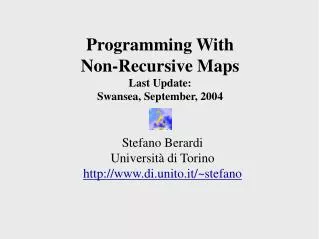
An example of D02-map • Denote by N®N the set of integer codes for total recursive maps over integers. • Using Classical Logic, we may prove there is a map F:(N®N)®N, picking, for any f:N®N, some m = F(f) which is a minimum point for f: "xÎN. f(m) £ f(x) 7

An example of D02-map Here is m=F(f): y y=f(x) y=f(m) x=m x 8

F is not recursive There is no way of finding the minimum point m of f just by looking through finitely may values of f. y y=f(x) Area explored by a recursive F x m 9

D02-maps solve equations faster • Fix any three f, g, h:N®N. • Suppose we want to solve in x the unequation system: f(x) £ f(g(x)) f(x) £ f(h(x)) • x=F(f) is a solution: by the choice of x, we have f(x) £ f(y) for all yÎN, in particular for y=g(x), h(x). (1) 10

Did we really find a solution? • Using the D02-map F, we solved the system rather quickly, with x=F(f). • The solution x=F(f), however, cannot be computed. • Apparently, using non-recursive maps we only prove the existence of the solution. 11

Blind Search • The only evident way to find the solution is blind search: to look for the first xÎN such that f(x) £ f(g(x)) f(x) £ f(h(x)) • This is rather inefficient in general. • It makes no use of the ideas of the proof. (1) 12

Our Goal We want to define approximations of D02-maps, in order to use them to solve problems like the previous system. 13

2. Dynamic Objects Truth may change with time … 14

An Oracle for Simply Existential Statements • Our first step towards a model of D02-maps is: • to define, for any recursive map f:N®N, some approximation of an oracle O(f)Î{True,False} for $xÎN.f(x)=0. • O is no recursive map. • What do we know about $xÎN.f(x)=0 in general? 15

What do we know about $xÎN.f(x)=0? • We have, in general, an incomplete knowledge about $xÎN.f(x)=0. • Assume that, for some x1, ..., xn, we checked if f(x1)=0, ..., f(xn)=0 • If the answer is sometimes yes, we do know: $xÎN.f(x)=0 is True. • If the answer is always no, all we do know is: $xÎ{x1, ..., xn}.f(x)=0 is false 16

The idea: introducing a new object • Since we cannot compute the truth value of $xÎN.f(x)=0, we represent it by introducing a new object: the family of all incomplete computations of $xÎN.f(x)=0. • That is: the family of truth values of all $xÎ{x1, ..., xn}.f(x)=0 • for {x1, ..., xn} finite set of integers. 17

A notion of State • We formalize the idea of incomplete computation of the truth value of $xÎN.f(x)=0 by introducing a set T of computation states or “instants of time”. • T is any partial ordering. • Each tÎT is characterized by a set a(t) of actions, taking place before t. In our case: a(t)={x1, ..., xn} • Any “action” corresponds to some xÎN for which we checked whether f(x)=0. 18

The truth value for $xÎN.f(x)=0 • The “truth value” V of $xÎN.f(x)=0 is a family: {V(t)}tÎT indexed over computation states, with V(t) = truth value of ($xÎa(t).f(x)=0). • The statement($xÎa(t).f(x)=0) is the restriction of ($xÎN.f(x)=0) to the finite set a(t)ÍN associated to t. 19

In each tT, we compute f(x) for some new x u3 f(9)=0 V(u3)=T T v3 v2 u2 V(u2)=F f(6)=6 f(5)=7 V(v3)=F t3 f(8)=2 V(t3)=T u1 f(2)=11 V(u1)=F V(t2)=T v1 f(4)=0 t2 f(8)=2 V(v2)=F t1 V(t1)=F f(5)=7 f(3)=1 V(t0)=V(u0)=V(v0)=F t0=u0=v0 20

3. Event Structures We record all we did … 21

A notion of Event Structure An Event Structure consists of: 1. An inhabited recursive partial ordering Tof states. 2. a recursive set A of actions, which we may execute in any state tÎT, and whichmay fail. 3. A recursive map a:T®{finite subsets of A} a(t) = set of all actions executed before state t a is weakly increasing. 22

Covering Assumption Every action may be executed in any state: for any tÎT, xÎA, there is some possibly future u³t such that xÎa(u) (x is executed before u). T (states) action x is executed here (it may fail) u t 23

An example of Event Structure We consider actions of the form <d,i>: “send the datum d to the memory of name i”. A (actions) = Data  MemoryNames T (states) = List(A) a(t) (actions before t) = {<d,i> | <d,i>t} Any tÎT describes a computation up to the state t. Most of the information in t is intended only as comment to the computation.

Positive Informations • Assume <d,i>a(t): we sent datum d to the memory i before state t. • Then d is paired with i in all possible futures u of t (in all ut), because a is weakly increasing. • In Event Structure we represent only positive informations: erasing is not a primitive operation. • Erasing may be represented by using a fresh name for any new state of the memory i: <i,0>, <i,1>, <i,2>, …

Erasing in Event Structures • When memory i is in the state number n, its current content are only all d such that < d, <i,n> >  a(t) • When the state number changes, the current content d of memory i is lost forever. • Every action a = <d, <i,m>> referring to a state m different from the current state(with mn) “fails” (by this we mean: a is recorded, but d is never used).

Dynamic Objects • Fix any recursive set X. • We call any recursive L:T®X a dynamic object over X • Dyn(X) = {dynamic objects over X} • Dyn(Bool) is the set of dynamic booleans. • The value of a dynamic object may change with time, and it may depends on all data we sent to any memory. 27

Embedding X in Dyn(X) • Static objects (objects whose value does not change with time) are particular dynamic objects. • There is an embedding (.)°:X®Dyn(X), mapping each xÎX into the dynamic object x°ÎDyn(X), defined by x°(t) = x for all tÎT 28

Morphisms over Dynamic Objects • Fix any recursive sets X, X’, Y. Any recursive application f : X, X’®Y may be raised pointwise to a recursive application: f° : Dyn(X), Dyn(X’) ® Dyn(Y) defined by f°(L)(t) = f(L(t)), for all tÎT. For instance we set: (L +° M)(t) = L(t) + M(t) • We consider all maps of the form f° as morphisms over dynamic objects. 29

Morphisms over Dynamic Objects • A morphism over dynamic objects should take the current value L(t) Î X of a dynamic object and return the current value f(L(t)) Î Y of another one • In general, however, f(L(t)) could be itself dynamic, that is, it could depend on time. • The same value L(t) could correspond to different values f(L(t)) for different t. • Thus, a morphism will be, in general, some map L, t  f(L(t))(t) 30

Morphisms over Dynamic Objects Fix any recursive sets X, Y. We call an application : Dyn(X)®Dyn(Y) a morphism if (L)(t) depends only over the current value L(t) of L, and on tÎT: ( L )(t) = ( L(t)° )(t) for all tÎT 31

Raising a map to a morphism • For all recursive X, Y, every recursive f:X® Dyn(Y) may be raised to a unique morphism f* :Dyn(X) ® Dyn(Y) • Set, for all tÎT, and all LÎDyn(X): f*(L)(t) = f(L(t))(t) ÎY • f*(L) is called a synchronous application: the output f(.)(t) and the input L(t) have the same clock tÎT 32

X Y f* L(t2) f(L(t2))(t2) f* L(t1) f(L(t1))(t1) f* L(t0) f(L(t0))(t0) 33

4. Convergence and Equality for Dynamic Objects We interpret parallel computations in Event Structures. 34

Some terminology for Parallel Computations • Computation states.They include local states of processes, and the state of a common memory. • Computation. An asyncronous parallel execution for a finite set of processes. • Agents. Processes modifying the common memory. • Clusters of Agents .Finite sets of agent, whose composition may change with time. 35

Interpreting Computation States • Any tÎT describes a possible state of a computation. • Any weakly increasing succession t:N®T represents a possible history of a computation. 36

Interpreting Computations A computation is any weakly increasing total recursive succession t:N®T of states. T (states) t(3) t(2) t(1) t(0) 37

Execution of an Agent • An agent outputs actions, possibly at very long intervals of time. • Any action may take very long time to be executed. • We allow actions to be executed in any order. • Many other actions, from different agents, may be executed at the same time: there is no priority between agent. 38

Interpreting Agents • A agent is a way of choosing the next state in a computation. • A agent is any total recursive map A : T®A • taking an state t, and returning some action A(t)ÎA to execute from t. • If t is any computation, we define the set of actions of t by nNa(t(n)) 39

Computations executing an Agent We say that a computation t:N®T executes a agent A, or t:A for short, iff for infinitely many iÎN: A(t(i)) {actions of t} That is: for infinitely many times, the action output by A at some step of t are executed in some step in t (maybe much later) If t:F, and  is subsuccession of t, we set by definition:F. 40

Computations executing an Agent If a computation t executes a agent A, then A “steers” t: for infinitely many times, the next position in t is partly determined by the action output by A. T (states) t(3) t(2) Constraint: a(t(2))  A(t(1)) t(1) t(0) 41

Computations executing many Agents Many agents A, B, C, … may “steer” infinitely many times the same computation t: T (states) Constraint: a(t(4))  C(t(3)) t(4) t(3) t(2) Constraints: a(t(2))  A(t(1)), B( t(1)) t(1) t(0) 42

Interpreting Clusters of Agents • A cluster is a set of agents variable in time, represented by a total recursive map F : T®{finite sets of agents} • taking an state tÎT, and returning the finite set of agents which are part of the cluster in the state t. • The agent A corresponds to the cluster constantly equal to {A}. 43

Computation executing a Cluster We say that t executes a cluster F, or t:F, iff for all agents A there are infinitely many iÎN such that if AÎF(t(i)), then A (t(i)){actions of t} In infinitely many steps of t, provided A is currently inF, the action output by A takes place (maybe much later) in t If t:F, and  is subsuccession of a t, we set by definition:F. 44

Two Sets of of Computations • Let t:N®T be any computation, L, M:T®X any dynamic objects. • L is the set of computations t:N®T such that Lt(n) = Lt(n+1) : X, for some nN • (L=M) is the set of computations t:N®T such that Lt(n) = Mt(n) : X, for some nN 45

Forcing We say that a cluster F forces a set P of computations, and we write F : P iff t:Fimplies tP (if all computations executing F have the property P). 46

Convergence and Equality for Dynamic Objects Let L, M:T®X be any dynamic objects. L is convergent iff F : L for some F L,Mare equivalent iff F : (L=M) for some F We think of a convergent dynamic object as a process “learning” a value. Let P: T®Bool be any dynamic boolean. P is true iff F:(P=True°) for some F 47

AssumeA:L A “steers” t, forcing L … Constraint: a(t(6)) A(t(5)) t(6) L(t(6))=13 t(5) L(t(5))=13 t(4) L(t(4))=13 t(3) Constraint: a(t(2)) A(t(1)) t(2) t(1) t(0) 48

About Convergence Assume F forces L to converge. Classically, we may prove that if t:F, then Lt is stationary. However: • On two different computations following F, L may converge to different values. • On some computation not following F, L may diverge.

u : F  Lu is convergent t : F  Lt is convergent Lu(2)=4 Lr(2)=9 Lt(3)=3 Lu(1)=4 r does not follows F: Lr can diverge Lt(2)=3 Lr(1)=1 Lt(1)=2 Lt(0)=7 50

Programming With Non-Recursive Maps Last Update: Swansea, September, 2004