Download
1 / 12
120 likes | 189 Views
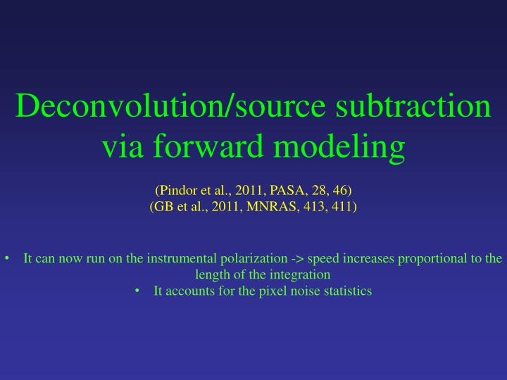
Deconvolution /source subtraction via forward modeling ( Pindor et al., 2011, PASA, 28, 46) (GB et al., 2011, MNRAS, 413, 411) It can now run on the instrumental polarization -> speed increases proportional to the length of the integration It accounts for the pixel noise statistics.

E N D
Deconvolution/source subtraction via forward modeling • (Pindor et al., 2011, PASA, 28, 46) (GB et al., 2011, MNRAS, 413, 411) • It can now run on the instrumental polarization -> speed increases proportional to the length of the integration • It accounts for the pixel noise statistics
Deconvolving real data: an example Source J0523-36 is modeled in the same way that the pointing is processed via the RTS (beams, cadence, frequency) Convergence after 2 iterations. Positional error ~ 15’, flux error ~ 10%
Primary beam measurements • the sky drifts overhead while the tiles point at zenith; • ~30 bandwidth centered @ 185 MHz; • snapshot images (one every 5 min) are used to measure the beam response towards the J0444-2905 (which is ~ 37 Jy @ 185 MHz);
Primary beam measurements J0444-2905
Fitting a simple primary beam model The beam is accurate at a 2% level and predicts the source fluxex with 5% rms accuracy
Stokes I The rms is 0.63 Jy/beam
Stokes Q The rms is 41 mJy/beam
Stokes U The rms is 28 mJy/beam
Extending the beam work: zooming in to HydA field HydA Observations span slightly more than 5 hours (total) over 110-200 MHz: 21 tiles available HydA provides the direction independent calibration of the array Snapshot images co-added Multi-frequency synthesis (but in the image plane)
to be continued with existing data with X16