Download
1 / 16
160 likes | 269 Views
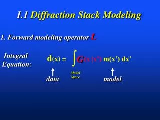
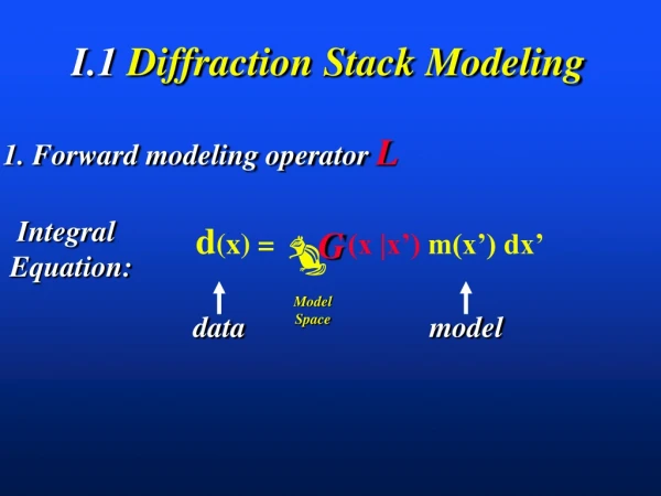
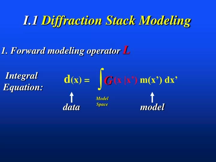
d (x) = (x |x’) m(x’) dx’. G. Integral Equation:. ò. model. data. Model Space. I.1 Diffraction Stack Modeling. 1. Forward modeling operator L. 2-way time. Forward Modeling. 2-way time. Forward Modeling: Sum of Weighted Hyperbolas. iw|x- x’ |/c . Phase. e .

E N D
d(x) = (x |x’) m(x’) dx’ G Integral Equation: ò model data Model Space I.1 Diffraction Stack Modeling 1. Forward modeling operator L
2-way time Forward Modeling
2-way time Forward Modeling: Sum of Weighted Hyperbolas
iw|x-x’|/c Phase e |x-x’| Geom. Spread |x-x’| x x’ GREEN’s FUNCTION G(x|x’) =
iw|x-x’|/c Phase xx’ xx’ e -1 + O( ) |x-x’| Geom. Spread x x’ ASYMPTOTIC GREEN’s FUNCTION G(x|x’) = A(x,x’)
i xx’ R(x’) x’ x’ reflectivity ASYMPTOTIC GREEN’s FUNCTION e G(x|x’) = A(x,x’)
1-way time Diffraction Stack Modeling = ZO Modeling
2-way time Diffraction Stack Modeling = ZO Modeling Dipping Reflector
1-way time Diffraction Stack Modeling = ZO Modeling If c for DS is ½ that for ZO Modeling
i i xx’ xx’ R(x’) x’ x’ reflectivity Fourier Transform: F e (t- ) xx’ (t- ) ~ F xx’ d(x) R(x’) A(x,x’) ASYMPTOTIC GREEN’s FUNCTION ~ e d(x) = A(x,x’)
QUICK REVIEW FOURIER TRANSFORM ( - t) xx’ i e d t Cos( 4 t ) + + (t- ) Cos( 2 t ) xx’ + Cos( 3 t ) cancellation cancellation Cos( t ) constructive reinforcement @ t=0 (t)
x’ time Sum over reflectivity Spray energy along hyperbolas (t- ) xx’ (t- ) xx’ Forward Modeling Operator d(x,t) = R(x’) A(x,x’)
W x’ time CANCELLATION REINFORCE (t- ) xx’ Forward Modeling Operator d(x,t) = R(x’) A(x,x’)
SUMMARY x’ d(x) = (x |x’)m(x’) dx’ G Integral Equation: reflectivity ò Source wavelet Geom. spreading model data Model Space W (t- ) xx’ 1. Exploding Reflector Modeling = Diffraction Stack Modeling R(x’) d(x,t) = Sum over reflectors Data variables A(x,x’) 2. High Frequency Approximation (i.e c(x) variations > 3* ) 3. Approximates Kinematics of ZO Sections, but not Dynamics
x’ d(x,t|x’,0) = R(x’) W (t- ) xx’ MATLAB Exercise: Forward Modeling 1. To account for the source wavelet W(t), we convolve data with W(t)(recall (t- )*W(t)= W() ) so that modeling equation becomes (neglect A) A). Execute MATLAB program forw.m to generate synthetic data for a point scatterer and a 30 Hz wavelet. B). Execute MATLAB program forwl.m to generate synthetic data for a dipping layer model C). Execute MATLAB program forw.m to generate synthetic data for a syncline model. Note diffractions and multiple arrivals. Adjust for new models. Why the second time derivative?
x’ d(x,t) = R(x’) Loop over traces Loop over x in model Loop over z in model Traveltime { W (t- ) R(x’) xx’ MATLAB Exercise: Forward Modeling for ixtrace=1:ntrace; for ixs=istart:iend; for izs=1:nz; r = sqrt((ixtrace*dx-ixs*dx)^2+(izs*dx)^2); time = 1 + round( r/c/dt ); data(ixtrace,time) = migi(ixs,izs)/r + data(ixtrace,time); end; end; data1(ixtrace,:)=conv2(data(ixtrace,:),rick); end; * Src Wave