Download
1 / 18
220 likes | 609 Views
Population Modeling. Mathematical Biology Lecture 2 James A. Glazier (Partially Based on Brittain Chapter 1). Population Models. Simple and a Good Introduction to Methods Two Types Continuum [Britton, Chapter 1] Discrete [Britton, Chapter 2]. Continuum Population Models.

E N D
Population Modeling Mathematical Biology Lecture 2 James A. Glazier (Partially Based on Brittain Chapter 1)
Population Models Simple and a Good Introduction to Methods Two Types • Continuum [Britton, Chapter 1] • Discrete [Britton, Chapter 2]
Continuum Population Models • Given a Population, N0 of an animal, cell, bacterium,… at time t=0, What is the Population N(t) at time t? Assume that the population is large so treat Nas a continuous variable. • Naively: • Continuum Models are Generally More Stable than discrete models (no chaos or oscillations)
Malthusian Model (Exponential Growth) • For a Fertility Rate, b, a Death Rate,d, and no Migration: In reality have a saturation: limited food, disease, predation, reduced birth-rate from crowding…
Density Dependent Effects • How to Introduce Density Dependent Effects? • Decide on Essential Characteristics of Data. • Write Simplest form of f(N) which Gives these Characteristics. • Choose Model parameters to Fit Data • Generally, Growth is Sigmoidal, i.e. small for small and large populations f(0) = f(K) = 0, where Kis the Carrying Capacity and f(N) has a unique maximum for some value of N, Nmax • The Simplest Possible Solution is the Verhulst or Logistic Equation
Verhulst or Logistic Equation • A Key Equation—Will Use Repeatedly • Assume Death Rate N, or that Birth Rate Declines with IncreasingN, Reaching 0 at the Carrying Capacity, K: • The Logistic Equation has a Closed-Form Solution: No Chaos in Continuum Logistic Equation Click for Solution Details
Solving the Logistic Equation 2) Now let: 1) Start with Logistic Equation: 3) Substitute: 4) Solve for N(t):
General Issues in Modeling • Not a model unless we can explain why the death rate d~N/K. • Can always improve fit using more parameters. • Meaningless unless we can justify them. • Logistic Map has only three parameters N0, K, r – doesn't fit real populations, very well. But we are not just curve fitting. • Don't introduce parameters unless we know they describe a real mechanism in biology. • Fitting changes in response to different parameters is much more useful than fitting a curve with a single set of parameters.
Idea: Steady State or Fixed Point • For a Differential Equation of Form • is a Fixed Point • So the Logistic Equation has Two Fixed Points, N=0 and N=K • Fixed Points are also often designated x*
Idea: Stability • Is the Fixed Point Stable? • I.e. if you move a small distance e away from x0 does x(t) return to x0? • If so x0 is Stable, if not, x0 is Unstable.
Calculating Stability: Linear Stability Analysis • Consider a Fixed Point x0 and a Perturbation e. Assume that: • Taylor Expand f around x0: • So, if Response Timescale, t, for disturbance to grow or shrink by a factor of eis:
Example Logistic Equation Start with the Logistic Eqn. Fixed Points at N0=0 and N0=K For N0=0 unstable For N0=K stable
Phase Portraits • Idea: Describe Stability Behavior Graphically Arrows show direction of Flow Generally:
Solution of the Logistic Equation Solution of the Logistic Equation: For N0>K, N(t) decreases exponentially to K For N0<2, K/N(t) increases sigmoidally to K For K/2<N0<K, N(t) increases exponentially to K
Example Stability in Population Competition Consider two species, N1 and N2, with growth rates r1 and r2 and carrying capacities K1 and K2, competing for the same resource. Both obey Logistic Equation. If one species has both bigger carrying capacity and faster growth rate, it will displace the other. What if one species has faster growth rate and the other a greater carrying capacity? An example of a serious evolutionary/ecological question answerable with simple mathematics.
Population Competition—Contd. Start with all N1 and no N2. Represent population as a vector (N1, N2) Steady state is (K1,0). What if we introduce a few N2? In two dimensions we need to look at the eigenvalues of the Jacobian Matrix evaluated at the fixed point. Evaluate at (K1,0).
Stability in Two Dimensions Cases: 1) Both Eigenvalues Positive—Unstable 2) One Eigenvalue Positive, One Negative—Unstable 1) Both Eigenvalues Negative—Stable
Population Competition—Contd. Eigenvalues are solutions of -r1 always < 0 so fixed point is stable r2(1-K1/K2)<0i.e. if K1>K2. Fixed Point Unstable (i.e. species 2 Invades Successfully) K2>K1 Independent of r2! So high carrying capacity wins out over high fertility (called K-selection in evolutionary biology). A surprising result. The opposite of what is generally observed in nature.