Download
1 / 81
830 likes | 840 Views
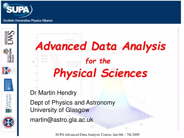
Advanced Data Analysis for the Physical Sciences. Dr Martin Hendry Dept of Physics and Astronomy University of Glasgow martin@astro.gla.ac.uk. SUPA Advanced Data Analysis Course, Jan 6th – 7th 2009. SUPA Advanced Data Analysis Course, Jan 6th – 7th 2009.

E N D
Advanced Data Analysis for the Physical Sciences Dr Martin Hendry Dept of Physics and Astronomy University of Glasgow martin@astro.gla.ac.uk SUPA Advanced Data Analysis Course, Jan 6th – 7th 2009
SUPA Advanced Data Analysis Course, Jan 6th – 7th 2009 3. Parameter Estimation and Goodness of Fit – Part Two In the previous section we have discussed how to estimate parameters of an underlying pdf model from sample data. We now consider the closely related question: How good is our pdf model in the first place?
SUPA Advanced Data Analysis Course, Jan 6th – 7th 2009 3. Parameter Estimation and Goodness of Fit – Part Two In the previous section we have discussed how to estimate parameters of an underlying pdf model from sample data. We now consider the closely related question: How good is our pdf model in the first place? Simple Hypothesis test – example. Null hypothesis: sampled data are drawn from a normal pdf, with mean and variance . We want to test this null hypothesis: are our data consistent with it?
SUPA Advanced Data Analysis Course, Jan 6th – 7th 2009 Assume (for the moment) that is known. Example Measured data: Null hypothesis: with Assume: Under NH, sample mean Observed sample mean
SUPA Advanced Data Analysis Course, Jan 6th – 7th 2009 We transform to a standard normal variable Under NH: From our measured data: If NH is true, how probable is it that we would obtain a value of as large as this, or larger? We call this probability thep-value
SUPA Advanced Data Analysis Course, Jan 6th – 7th 2009 p-value Simple programs to perform this probability integral (and many others) can be found in numerical recipes, or built into e.g. MATLAB or MAPLE. Java applets also available online at http://statpages.org/pdfs.html
SUPA Advanced Data Analysis Course, Jan 6th – 7th 2009 p-value The smallerthe p-value, the less credible is the null hypothesis.
SUPA Advanced Data Analysis Course, Jan 6th – 7th 2009 p-value The smallerthe p-value, the less credible is the null hypothesis. (We can also carry out a one-tailed hypothesis test, if appropriate, and for statistics with other sampling distributions).
Question 6: A one-tailed hypothesis test is carried out. Under the NH the test statistic has a uniform distribution . The observed value of the test statistic is 0.8. The p-value is: A 0.8 B 0.9 C 0.2 D 0.1
Question 6: A one-tailed hypothesis test is carried out. Under the NH the test statistic has a uniform distribution . The observed value of the test statistic is 0.8. The p-value is: A 0.8 B 0.9 C 0.2 D 0.1
SUPA Advanced Data Analysis Course, Jan 6th – 7th 2009 What if we don’t assume that is known? We can estimate it from our observed data (provided ) We form the statistic where However, now no longer has a normal distribution. Accounts for the fact that we don’t know , but must use when we estimate
SUPA Advanced Data Analysis Course, Jan 6th – 7th 2009 In fact has a pdf known as the Student’s t distribution where is the no. degrees of freedom and For small the Student’s t distribution has more extended tails than , but as the distribution tends to
Question 7: The more extended tails of the students’ t distribution mean that, under the null hypothesis A larger values of the test statistic are more likely B larger values of the test statistic are less likely C smaller values of the test statistic are more likely D smaller values of the test statistic are less likely
Question 7: The more extended tails of the students’ t distribution mean that, under the null hypothesis A larger values of the test statistic are more likely B larger values of the test statistic are less likely C smaller values of the test statistic are more likely D smaller values of the test statistic are less likely
SUPA Advanced Data Analysis Course, Jan 6th – 7th 2009 3. Parameter Estimation and Goodness of Fit – Part Two More generally, we now illustrate the frequentist approach to the question of how good is the fit to our model, using the Chi-squared goodness of fit test. We take an example from Gregory (Chapter 7) (book focusses mainly on Bayesian probability, but is very good on frequentist approach too)
SUPA Advanced Data Analysis Course, Jan 6th – 7th 2009 Model: radio emission from a galaxy is constant in time. Assume residuals are iid, drawn from N(0,)
SUPA Advanced Data Analysis Course, Jan 6th – 7th 2009 Goodness-of-fit Test: the basic ideas From Gregory, pg. 164
SUPA Advanced Data Analysis Course, Jan 6th – 7th 2009 The 2 pdf
SUPA Advanced Data Analysis Course, Jan 6th – 7th 2009 n = 15 data points, but = 14 degrees of freedom, because statistic involves the sample mean and not the true mean. We subtract one d.o.f. to account for this.
n = 15 data points, but = 14 degrees of freedom, because statistic involves the sample mean and not the true mean. We subtract one d.o.f. to account for this. If the null hypothesis is true, how probable is it that we would measure as large, or larger, a value of ?
SUPA Advanced Data Analysis Course, Jan 6th – 7th 2009 If the null hypothesis were true, how probable is it that we would measure as large, or larger, a value of ? Recall that we refer to this important quantity as the p-value
If the null hypothesis were true, how probable is it that we would measure as large, or larger, a value of ? Recall that we refer to this important quantity as the p-value What precisely does the p-value mean? If we obtain a very small p-value (e.g. a few percent?) we can interpret this as providing little support for the null hypothesis, which we may then choose to reject. (Ultimately this choice is subjective, but may provide objective ammunition for doing so) “If the galaxy flux density really is constant, and we repeatedly obtained sets of 15 measurements under the same conditions, then only 2% of the values derived from these sets would be expected to be greater than our one actual measured value of 26.76” From Gregory, pg. 165
If the null hypothesis were true, how probable is it that we would measure as large, or larger, a value of ? Recall that we refer to this important quantity as the p-value What precisely does the p-value mean? “If the galaxy flux density really is constant, and we repeatedly obtained sets of 15 measurements under the same conditions, then only 2% of the values derived from these sets would be expected to be greater than our one actual measured value of 26.76” From Gregory, pg. 165 “At this point you may be asking yourself why we should care about a probability involving results never actually obtained” From Gregory, pg. 166
SUPA Advanced Data Analysis Course, Jan 6th – 7th 2009 Nevertheless, p-value based frequentist hypothesis testing remains very common in the literature: Type of problem test References Line and curve NR: 15.1-15.6 goodness-of-fit Difference of means Student’s t NR: 14.2 Ratio of variances F test NR: 14.2 Sample CDF K-S test NR: 14.3, 14.6 Rank sum tests Correlated variables? Sample correlation NR: 14.5, 14.6 coefficient Discrete RVs test / NR: 14.4 contingency table test
SUPA Advanced Data Analysis Course, Jan 6th – 7th 2009 Nevertheless, p-value based frequentist hypothesis testing remains very common in the literature: Type of problem test References Line and curve NR: 15.1-15.6 goodness-of-fit Difference of means Student’s t NR: 14.2 Ratio of variances F test NR: 14.2 Sample CDF K-S test NR: 14.3, 14.6 Rank sum tests Correlated variables? Sample correlation NR: 14.5, 14.6 coefficient Discrete RVs test / NR: 14.4 contingency table test See also supplementary notes on my.SUPA
Prior Likelihood Posterior Influence of our observations What we knew before What we know now SUPA Advanced Data Analysis Course, Jan 6th – 7th 2009 In the Bayesian approach, we can test our model, in the light of our data (e.g. rolling a die) and see how our knowledge of its parameters evolves, for any sample size, considering only the data that we did actually observe
Prior Likelihood Posterior Influence of our observations What we knew before What we know now SUPA Advanced Data Analysis Course, Jan 6th – 7th 2009 In the Bayesian approach, we can test our model, in the light of our data (e.g. rolling a die) and see how our knowledge of its parameters evolves, for any sample size, considering only the data that we did actually observe Astronomical example: Probability that a galaxy is a Seyfert 1
SUPA Advanced Data Analysis Course, Jan 6th – 7th 2009 We want to know the fraction of Seyfert galaxies which are type 1. How large a sample do we need to reliably measure this?
SUPA Advanced Data Analysis Course, Jan 6th – 7th 2009 We want to know the fraction of Seyfert galaxies which are type 1. How large a sample do we need to reliably measure this? Model as a binomial pdf: = global fraction of Seyfert 1s Suppose we sample N Seyferts, and observe r Seyfert 1s Likelihood = probability of obtaining observed data, given model
Prior Likelihood Posterior Influence of our observations What we knew before What we know now SUPA Advanced Data Analysis Course, Jan 6th – 7th 2009 We want to know the fraction of Seyfert galaxies which are type 1. How large a sample do we need to reliably measure this? Model as a binomial pdf: = global fraction of Seyfert 1s Suppose we sample N Seyferts, and observe r Seyfert 1s Likelihood = probability of obtaining observed data, given model
SUPA Advanced Data Analysis Course, Jan 6th – 7th 2009 What do we choose as our prior? Good question!! Source of much argument between Bayesians and frequentists Blood on the walls
Prior Likelihood Posterior SUPA Advanced Data Analysis Course, Jan 6th – 7th 2009 What do we choose as our prior? Good question!! Source of much argument between Bayesians and frequentists If our data are good enough, it shouldn’t matter!! Blood on the walls Dominates
SUPA Advanced Data Analysis Course, Jan 6th – 7th 2009 From Gregory, pg 8.
Hubble’s Law: 1929 Hubble parameter = expansion rate of the Universe = slope of Hubble’s law
SUPA Advanced Data Analysis Course, Jan 6th – 7th 2009 • ‘Toy’ model problem: What is the relative • proportion of Seyfert 1 galaxies in the • Universe? • We can generate fake data to see how the influence of the likelihood and prior evolve. • Choose a ‘true’ value of • Sample a uniform random number, x, from [0,1] • (see Numerical Recipes, and Sect 6) • Prob( x < ) = • Hence, if x < Seyfert 1 • otherwise Seyfert 2 • Repeat from step 2
SUPA Advanced Data Analysis Course, Jan 6th – 7th 2009 • ‘Toy’ model problem: What is the relative • proportion of Seyfert 1 galaxies in the • Universe? • We can generate fake data to see how the influence of the likelihood and prior evolve. • Choose a ‘true’ value of • Sample a uniform random number, x, from [0,1] • (see Numerical Recipes, and Sect 6) • Prob( x < ) = • Hence, if x < Seyfert 1 • otherwise Seyfert 2 Take = 0.25 • Repeat from step 2
SUPA Advanced Data Analysis Course, Jan 6th – 7th 2009 Consider two different priors Flat prior; all values of equally probable p( |I ) Normal prior; peaked at = 0.5
SUPA Advanced Data Analysis Course, Jan 6th – 7th 2009 After observing 0 galaxies p( | data, I )
SUPA Advanced Data Analysis Course, Jan 6th – 7th 2009 After observing 1 galaxy: Seyfert 1 p( | data, I )
SUPA Advanced Data Analysis Course, Jan 6th – 7th 2009 After observing 2 galaxies: S1 + S1 p( | data, I )
SUPA Advanced Data Analysis Course, Jan 6th – 7th 2009 After observing 3 galaxies: S1 + S1 + S2 p( | data, I )
SUPA Advanced Data Analysis Course, Jan 6th – 7th 2009 After observing 4 galaxies: S1 + S1 + S2 + S2 p( | data, I )
SUPA Advanced Data Analysis Course, Jan 6th – 7th 2009 After observing 0 galaxies p( | data, I )
SUPA Advanced Data Analysis Course, Jan 6th – 7th 2009 After observing 4 galaxies: S1 + S1 + S2 + S2 p( | data, I )
SUPA Advanced Data Analysis Course, Jan 6th – 7th 2009 After observing 5 galaxies: S1 + S1 + S2 + S2 + S2 p( | data, I )
SUPA Advanced Data Analysis Course, Jan 6th – 7th 2009 After observing 10 galaxies: 5 S1 + 5 S2 p( | data, I )
SUPA Advanced Data Analysis Course, Jan 6th – 7th 2009 After observing 0 galaxies p( | data, I )
SUPA Advanced Data Analysis Course, Jan 6th – 7th 2009 After observing 10 galaxies: 5 S1 + 5 S2 p( | data, I )
SUPA Advanced Data Analysis Course, Jan 6th – 7th 2009 After observing 20 galaxies: 7 S1 + 13 S2 p( | data, I )
SUPA Advanced Data Analysis Course, Jan 6th – 7th 2009 After observing 50 galaxies: 17 S1 + 33 S2 p( | data, I )