Random samples and estimation

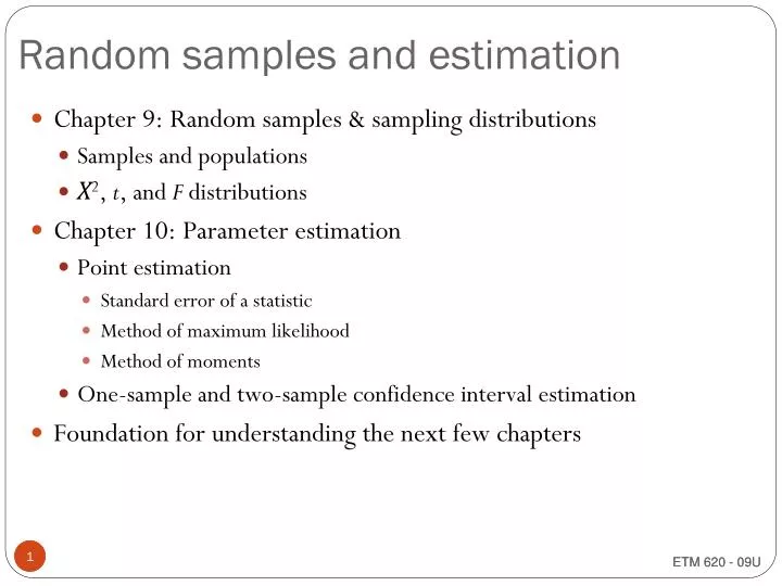
1. Random samples and estimation Chapter 9: Random samples & sampling distributions Samples and populations Χ2, t, and F distributions Chapter 10: Parameter estimation Point estimation Standard error of a statistic Method of maximum likelihood Method of moments One-sample and two-sample confidence interval estimation Foundation for understanding the next few chapters 1 ETM 620 - 09U

2. Ch. 9: Populations and samples • Population: “a group of individual persons, objects, or items from which samples are taken for statistical measurement” • Sample: “a finite part of a statistical population whose properties are studied to gain information about the whole” (Merriam-Webster Online Dictionary, http://www.m-w.com/, October 5, 2004) 2 ETM 620 - 09U

3. Population Students pursuing graduate engineering degrees Cars capable of speeds in excess of 160 mph. Potato chips produced at the Frito-Lay plant in Kathleen Freshwater lakes and rivers Samples Examples • In general, (x1, x2, x3, …, xn)are random samples of size n if: • the x’s are independent random variables • every observation is equally likely (has the same probability) 3 ETM 620 - 09U

4. Sampling distributions • If we conduct the same experiment several times with the same sample size, the probability distribution of the resulting statistic is called a sampling distribution • Sampling distribution of the mean: if n observations are taken from a normal population with mean μand variance σ2, then: 4 ETM 620 - 09U

5. An important consideration … • will be different for every sample • For example, suppose we know the time to complete a typical homework problem, in minutes, is known to be uniformly distributed between 5 and 25. Four people are asked to record the time it takes them to complete each of 31 different problems. 5 ETM 620 - 09U

6. Individual data points • μ = __________________ • σ2 = _________________ • σ= __________________ 6 ETM 620 - 09U

7. Sample means • = __________________ • = _________________ • = __________________ 7 ETM 620 - 09U

8. Central Limit Theorem • Given: • X :the mean of a random sample of size n taken from a population with mean μ and finite variance σ2, • Then, • the limiting form of the distribution of is _________________________ 8 ETM 620 - 09U

9. Central Limit Theorem • If the population is known to be normal, the sampling distribution of X will follow a normal distribution. • Even when the distribution of the population is not normal, the sampling distribution of X is normal when n is large. • NOTE: when n is not large, we cannot assume the distribution of X is normal. 9 ETM 620 - 09U

10. Sampling distribution of S2 : Χ2 • Given: • Z12, Z22, … , Zk2normally distributed random variables, with mean μ and standard deviation σ = 1. • Then, follows a χ2 distribution with k degrees of freedom and distribution function, (eq. 9-15, pg. 208) • μ = k σ2 = 2k 10 ETM 620 - 09U

11. χ2 Distribution • χα2represents the χ2value above which we find an area of α, that is, for which P(χ2> χα2) = α. • In Excel, =CHIDIST(x,degrees_freedom) • χ2is additive, so if Y =∑ χi2, then kY =∑ki • Sample variance, 11 ETM 620 - 09U

12. Student’s t Distribution • If Z ~N(0,1) and V is a chi-square random variable with k degrees of freedom, then follows a t-distribution with k degrees of freedom. The probability density function is, 12 ETM 620 - 09U

13. t- Distribution • Example 9-7 shows that follows a t distribution. In other words, x ~t(n-1) when σ is not know but is estimated by s. • In Excel, =TDIST(x,degrees_freedom,tails) gives the probability associated with getting a value above x (tails = 1) or outside +x (tails =2). =TINV(probability,degrees_freedom) gives the value associated with a desired probability,α. 13 ETM 620 - 09U

14. F-Distribution • Given: • S12 and S22, the variances of independent random samples of size n1 and n2taken from normal populations with variances σ12 and σ22, respectively, • Then, follows an F-distribution with ν1 = n1 - 1 and ν2 = n2 – 1 degrees of freedom. • Table V, pp 605-609 gives F-values associated with given α values. • In Excel, =FDIST(x,degrees_freedom1,degrees_freedom2) gives probability associated with a given x-value, while =FINV(probability,degrees_freedom1,degrees_freedom2) gives F-value associated with a given α. 14 ETM 620 - 09U

15. Ch. 10: Parameter estimation • Example: Say we have 5 numbers from a random sample, as follows: 19, 58, 31, 44, 43 • ̅x = ____________________ is an estimate of μ • s2 = _____________________ is an estimate of σ2 • We want to use “good” estimators (unbiased, minimum error) • Unbiased, i.e. E(̂θ) = θ(e.g., E(̅x) = ___, and E(S2) = __) • Minimum error, • MSE(θ̂ - θ) = E(θ̂ - θ)2 = Var(θ̂) 15 ETM 620 - 09U

16. Finding good estimators • Method of maximum likelihood • take n random samples (x1, x2, x3, .., xn) from a distribution with function f(x,θ) • Likelihood function, L(θ) = f(x1,θ) ∙ f(x2,θ) ∙ f(x3,θ) ∙ ∙ ∙ f(xn,θ) • Take the derivative with respect to θand set to 0. • See example 10-4, pg. 222 • not always unbiased, but can be modified to make it so. • Method of moments • First k moments about the origin of any function is • Can produce good estimators, but sometimes not as good as MLE (for example). 16 ETM 620 - 09U

17. Interval estimation • (1 – α)100% confidence interval for the unknown parameter • For some statistic, θ(e.g., μ) looking for L and U such that P{L <θ< U} = 1 – α or _______________ or ________________ ETM 620 - 09U

18. Single sample: Estimating the mean Given: σ is known and X is the mean of a random sample of size n, Then, the (1 – α)100% confidence interval for μ is given by 18 ETM 620 - 09U

19. Example: mean with known variance A random sample of size 25 is taken from a normal distribution with unknown mean and known variance of 4 (i.e., N(μ,4)). X of the sample is determined to be 13.2. What is the 90% confidence interval around the mean? 19 ETM 620 - 09U

20. What does this mean? • Measure of the precision of the estimate • Length of the interval is a function of • confidence level • variance • sample size • Can vary n to decrease the length of the interval for the same confidence level. • For our example, suppose we want an error of 0.25 or less. Then, n = ___________________________________________ 20 ETM 620 - 09U

21. What if σ2is unknown? • If n is sufficiently large (> _______), then the large sample confidence interval is: • Otherwise, must use the t-statistic … 21 21 EGR 252 - Ch. 9

22. Single sample estimate of the mean(σ unknown, n not large) • Given: • σ is unknown and X is the mean of a random sample of size n (where n is not large), • Then, • the (1 – α)100% confidence interval for μ is given by 22 22 EGR 252 - Ch. 9

23. Example A traffic engineer is concerned about the delays at an intersection near a local school. The intersection is equipped with a fully actuated (“demand”) traffic light and there have been complaints that traffic on the main street is subject to unacceptable delays. To develop a benchmark, the traffic engineer randomly samples 25 stop times (in seconds) on a weekend day. The average of these times is found to be 13.2 seconds, and the sample variance, s2, is found to be 4 seconds2. Based on this data, what is the 95% confidence interval (C.I.) around the mean stop time during a weekend day? 23 23 EGR 252 - Ch. 9

24. Example (cont.) X = ______________ s = _______________ α = ________________ α/2 = _____________ t0.025,24 = _____________ __________________ < μ < ___________________ 24 24 EGR 252 - Ch. 9

25. C.I. on the variance • Given that is ~ Χ2with n-1 degrees of freedom. • then, gives the 100(1-α)% two-sided confidence interval on the variance. 25 ETM 620 - 09U

26. Confidence interval on a proportion • The proportion, P, in a binomial experiment may be estimated by • where X is the number of successes in n trials. • For a sample, the point estimate of the parameter is • The mean for the sample proportion is • and the sample variance is 26 ETM 620 - 09U

27. C.I. for proportions • An approximate (1-α)100% confidence interval for p is: • Large-sample C.I. for p1 – p2is: • Interpretation: _______________________________ 27 ETM 620 - 09U

28. Example 10.17 (pg. 240) n = 75 x = 12 z0.025= ________ Picture: C.I.: Interpretation: ____________________________________

29. Setting the sample size … • If the estimate for p from the initial estimate seems pretty reliable, then e.g., for our example if we want to be 95% confident that the error in our estimate is less than 0.05, then n = __________________ • If we’re not at all sure how to estimate p, then assume p = 0.5 and use

30. Example: comparing 2 proportions Look at example 10-23, pg. 250 C.I. = (-0.07, 0.15), therefore no reason to believe there is a significant decrease in the proportion defectives using the new process. What if the interval were (+0.07, 0.15)? What if the interval were (-0.9, -0.7)?

31. Difference in 2 means, both σ2 known • Given two independent random samples, a point estimate the difference between μ1 and μ2 is given by the statistic We can build a confidence interval for μ1 - μ2 (given σ12 and σ22 known) as follows: 31 31 ETM 620 - 09U

32. An example A farm equipment manufacturer wants to compare the average daily downtime of two sheet-metal stamping machines located in two different factories. Investigation of company records for 100 randomly selected days on each of the two machines gave the following results: ̅x1 = 12 minutes ̅x2 = 10 minutes 12 = 12 22 = 8 n1 = n2 = 100 Construct a 95% C.I. for μ1 – μ2 32 ETM 620 - 09U

33. Solution α/2 = _____________ z_____ = ____________ __________________ < μ1 – μ2 < _________________ Interpretation: Picture 33 ETM 620 - 09U

34. Differences in 2 means, σ2unknown • Case 1: σ12 and σ22 unknown but equal Where, 34 ETM 620 - 09U

35. Differences in 2 means, σ2unknown Case 2: σ12 and σ22 unknown and not equal Where, 35 ETM 620 - 09U

36. Example, σ2unknown • Suppose the farm equipment manufacturer was unable to gather data for 100 days. Using the data they were able to gather, they would still like to compare the downtime for the two machines. The data they gathered is as follows: x1 = 12 minutes x2 = 10 minutes s12 = 12 s22 = 8 n1 = 18 n2 = 14 Construct a 95% C.I. for μ1 – μ2assuming: • σ12 and σ22 unknown but equal • σ12 and σ22 unknown and not equal 36 ETM 620 - 09U

37. Solution: Case 1 t____ , ________= ____________ __________________ < μ1 – μ2 < _________________ Interpretation: Picture 37 ETM 620 - 09U

38. Your turn … • Solve Case 2 (assuming variances are not equal)

39. Paired Observations Suppose we are evaluating observations that are not independent … For example, suppose a teacher wants to compare results of a pretest and posttest administered to the same group of students. Paired-observation or Paired-sample test … Example: murder rates in two consecutive years for several US cities (see attached.) Construct a 90% confidence interval around the difference in consecutive years.

40. Solution D = ____________ tα/2, n-1 = _____________ a (1-α)100% CI for μDis: __________________ < μ1 – μ2 < _________________ Interpretation: Picture

41. C. I. for the ratio of two variances • If X1and X2are independent normal random variables with unknown and unequal means and variances, then the confidence interval on the ratio σ12/σ22 is given by: Note: for F-values not given in table V, recall that or use =FINV(probability,degrees_freedom1,degrees_freedom2)

42. Example 10-22 n1 = 12, s1= 0.85 n2 = 15, s2= 0.98 F____ , ____ , ____= ____________ F____ , ____ , ____= ____________ __________________ < σ12/σ22< _________________ Interpretation: Picture 42 ETM 620 - 09U