Download
1 / 125
1.35k likes | 1.66k Views
Chapter 10 Random Regressors and Moment-Based Estimation. Walter R. Paczkowski Rutgers University. Chapter Contents. 10.1 Linear Regression with Random x ’s 10.2 Cases in Which x and e are Correlated 10 .3 Estimators Based on the Method of Moments

E N D
Chapter 10 Random Regressors and Moment-Based Estimation Walter R. Paczkowski Rutgers University
Chapter Contents • 10.1 Linear Regression with Random x’s • 10.2 Cases in Which x and e are Correlated • 10.3 Estimators Based on the Method of Moments • 10.4 Specification Tests
10.1 Linear Regression with Random x’s
10.1 Linear Regression with Random x’s • Modified simple regression assumptions: • A10.1 yi = β1 + β2xi + ei correctly describes the relationship between yi and xiin the population, where β1 and β2 are unknown (fixed) parameters and ei is an unobservable random error term. • A10.2 The data pairs (xi, yi), i = 1, …, N, are obtained by random sampling. That is, the data pairs are collected from the same population, by a process in which each pair is independent of every other pair. Such data are said to be independent and identically distributed.
10.1 Linear Regression with Random x’s • Modified simple regression assumptions (Continued): • A10.3 The expected value of the error term e, conditional on the value of x, is zero. • If E(e|x) = 0, then we can show that it is also true that x and e are uncorrelated, and that cov(x, e) = 0. Explanatory variables that are not correlated with the error term are called exogenous variables. • Conversely, if x and e are correlated, then cov(x, e) ≠ 0 and we can show that E(e|x) ≠ 0. Explanatory variables that are correlated with the error term are called endogenous variables. • A10.4 In the sample, x must take at least two different values.
10.1 Linear Regression with Random x’s • Modified simple regression assumptions (Continued): A10.5 var(e|x) = σ2. The variance of the error term, conditional on any x, is a constant σ2. A10.6 The distribution of the error term is normal.
10.1 Linear Regression with Random x’s • Assumption A10.2 states that both y and x are obtained by a sampling process, and thus are random • This is the only one new assumption on our list
10.1 Linear Regression with Random x’s 10.1.1 The Small Sample Properties of the Least Squares Estimators • The result that under the classical assumptions, and fixed x’s, the least squares estimator is the best linear unbiased estimator, is a finite sample, or a small sample • This means is that the result does not depend on the size of the sample
10.1 Linear Regression with Random x’s 10.1.1 The Small Sample Properties of the Least Squares Estimators • Under assumptions A10.1–A10.6: • The least squares estimator is unbiased • The least squares estimator is the best linear unbiased estimator of the regression parameters, and the usual estimator of σ2 is unbiased • The distributions of the least squares estimators, conditional upon the x’s, are normal, and their variances are estimated in the usual way • The usual interval estimation and hypothesis testing procedures are valid
10.1 Linear Regression with Random x’s 10.1.1 The Small Sample Properties of the Least Squares Estimators • If x is random, as long as the data are obtained by random sampling and the other usual assumptions hold, no changes in our regression methods are required
10.1 Linear Regression with Random x’s 10.1.2 Large Sample Properties of the Least Squares Estimators • For the purposes of a ‘‘large sample’’ analysis of the least squares estimator, it is convenient to replace assumption A10.3 by: A10.3* E(e) = 0 and cov(x, e) = 0
10.1 Linear Regression with Random x’s 10.1.2 Large Sample Properties of the Least Squares Estimators • Now we can say: • Under assumptions A10.1, A10.2, A10.3*, A10.4, and A10.5, the least squares estimators: • Are consistent. • They converge in probability to the true parameter values as N→∞. • Have approximate normal distributions in large samples, whether the errors are normally distributed or not. • Our usual interval estimators and test statistics are valid, if the sample is large. • If assumption A10.3* is not true, and in particular if cov(x,e) ≠ 0 so that x and e are correlated, then the least squares estimators are inconsistent. • They do not converge to the true parameter values even in very large samples. • None of our usual hypothesis testing or interval estimation procedures are valid.
10.1 Linear Regression with Random x’s FIGURE 10.1 (a) Correlated x and e 10.1.3 Why Least Squares Estimation Fails
10.1 Linear Regression with Random x’s FIGURE 10.1 (b) Plot of data, true and fitted regression functions 10.1.3 Why Least Squares Estimation Fails
10.1 Linear Regression with Random x’s 10.1.3 Why Least Squares Estimation Fails • The statistical consequences of correlation between x and e is that the least squares estimator is biased — and this bias will not disappear no matter how large the sample • Consequently the least squares estimator is inconsistent when there is correlation between x and e
10.2 Cases in Which x and e are Correlated
10.2 Cases in Which x and e are Correlated • When an explanatory variable and the error term are correlated, the explanatory variable is said to be endogenous • This term comes from simultaneous equations models • It means ‘‘determined within the system’’ • Using this terminology when an explanatory variable is correlated with the regression error, one is said to have an ‘‘endogeneity problem’’
10.2 Cases in Which x and e are Correlated 10.2.1 Measurement Error • The errors-in-variables problem occurs when an explanatory variable is measured with error • If we measure an explanatory variable with error, then it is correlated with the error term, and the least squares estimator is inconsistent
10.2 Cases in Which x and e are Correlated 10.2.1 Measurement Error • Let y = annual savings and x* = the permanent annual income of a person • A simple regression model is: • Current income is a measure of permanent income, but it does not measure permanent income exactly. • It is sometimes called a proxy variable • To capture this feature, specify that: Eq. 10.1 Eq. 10.2
10.2 Cases in Which x and e are Correlated 10.2.1 Measurement Error • Substituting: Eq. 10.3
10.2 Cases in Which x and e are Correlated 10.2.1 Measurement Error • In order to estimate Eq. 10.3 by least squares, we must determine whether or not x is uncorrelated with the random disturbance e • The covariance between these two random variables, using the fact that E(e) = 0, is: Eq. 10.4
10.2 Cases in Which x and e are Correlated 10.2.1 Measurement Error • The least squares estimator b2 is an inconsistent estimator of β2 because of the correlation between the explanatory variable and the error term • Consequently, b2 does not converge to β2 in large samples • In large or small samples b2 is not approximately normal with mean β2 and variance
10.2 Cases in Which x and e are Correlated 10.2.2 Simultaneous Equations Bias • Another situation in which an explanatory variable is correlated with the regression error term arises in simultaneous equations models • Suppose we write: Eq. 10.5
10.2 Cases in Which x and e are Correlated 10.2.2 Simultaneous Equations Bias • There is a feedback relationship between P and Q • Because of this, which results because price and quantity are jointly, or simultaneously, determined, we can show that cov(P, e) ≠ 0 • The resulting bias (and inconsistency) is called the simultaneous equations bias
10.2 Cases in Which x and e are Correlated 10.2.3 Omitted Variables • When an omitted variable is correlated with an included explanatory variable, then the regression error will be correlated with the explanatory variable, making it endogenous
10.2 Cases in Which x and e are Correlated 10.2.3 Omitted Variables • Consider a log-linear regression model explaining observed hourly wage: • What else affects wages? What have we omitted? Eq. 10.6
10.2 Cases in Which x and e are Correlated 10.2.3 Omitted Variables • We might expect cov(EDUC, e) ≠ 0 • If this is true, then we can expect that the least squares estimator of the returns to another year of education will be positively biased, E(b2) > β2, and inconsistent • The bias will not disappear even in very large samples
10.2 Cases in Which x and e are Correlated 10.2.4 Least Squares Estimation of a Wage Equation • Estimating our wage equation, we have: • We estimate that an additional year of education increases wages approximately 10.75%, holding everything else constant • If ability has a positive effect on wages, then this estimate is overstated, as the contribution of ability is attributed to the education variable
10.3 Estimators Based on the Method of Moments
10.3 Estimators Based on the Method of Moments • When all the usual assumptions of the linear model hold, the method of moments leads to the least squares estimator • If x is random and correlated with the error term, the method of moments leads to an alternative, called instrumental variables estimation, or two-stage least squares estimation, that will work in large samples
10.3 Estimators Based on the Method of Moments 10.3.1 Method of Moments Estimation of a Population Mean and Variance • The kth moment of a random variable Y is the expected value of the random variable raised to the kth power: • Thekth population moment in Eq. 10.7 can be estimated consistently using the sample (of size N) analog: Eq. 10.7 Eq. 10.8
10.3 Estimators Based on the Method of Moments 10.3.1 Method of Moments Estimation of a Population Mean and Variance • The method of moments estimation procedure equates m population moments to m sample moments to estimate m unknown parameters • Example: Eq. 10.9
10.3 Estimators Based on the Method of Moments 10.3.1 Method of Moments Estimation of a Population Mean and Variance • The first two population and sample moments of Y are: Eq. 10.10
10.3 Estimators Based on the Method of Moments 10.3.1 Method of Moments Estimation of a Population Mean and Variance • Solve for the unknown mean and variance parameters: and Eq. 10.11 Eq. 10.12
10.3 Estimators Based on the Method of Moments 10.3.2 Method of Moments Estimation in the Simple Linear Regression Model • In the linear regression model y = β1 + β2x + e, we usually assume: • If x is fixed, or random but not correlated with e, then: Eq. 10.13 Eq. 10.14
10.3 Estimators Based on the Method of Moments 10.3.2 Method of Moments Estimation in the Simple Linear Regression Model • We have two equations in two unknowns: Eq. 10.15
10.3 Estimators Based on the Method of Moments 10.3.2 Method of Moments Estimation in the Simple Linear Regression Model • These are equivalent to the least squares normal equations and their solution is: • Under "nice" assumptions, the method of moments principle of estimation leads us to the same estimators for the simple linear regression model as the least squares principle Eq. 10.16
10.3 Estimators Based on the Method of Moments 10.3.3 Instrumental Variables Estimation in the Simple Linear Regression Model • Suppose that there is another variable, z, such that: • z does not have a direct effect on y, and thus it does not belong on the right-hand side of the model as an explanatory variable • z is not correlated with the regression error term e • Variables with this property are said to be exogenous • z is strongly [or at least not weakly] correlated with x, the endogenous explanatory variable A variable z with these properties is called an instrumental variable
10.3 Estimators Based on the Method of Moments 10.3.3 Instrumental Variables Estimation in the Simple Linear Regression Model • If such a variable z exists, then it can be used to form the moment condition: • Use Eqs. 10.13 and 10.16, the sample moment conditions are: Eq. 10.16 Eq. 10.17
10.3 Estimators Based on the Method of Moments 10.3.3 Instrumental Variables Estimation in the Simple Linear Regression Model • Solving these equations leads us to method of moments estimators, which are usually called the instrumental variable (IV) estimators: Eq. 10.18
10.3 Estimators Based on the Method of Moments 10.3.3 Instrumental Variables Estimation in the Simple Linear Regression Model • These new estimators have the following properties: • They are consistent, if z is exogenous, with E(ze) = 0 • In large samples the instrumental variable estimators have approximate normal distributions • In the simple regression model: Eq. 10.19
10.3 Estimators Based on the Method of Moments 10.3.3 Instrumental Variables Estimation in the Simple Linear Regression Model • These new estimators have the following properties (Continued): • The error variance is estimated using the estimator:
10.3 Estimators Based on the Method of Moments 10.3.3a The Importance of Using Strong Instruments • Note that we can write the variance of the instrumental variables estimator of β2 as: • Because the variance of the instrumental variables estimator will always be larger than the variance of the least squares estimator, and thus it is said to be less efficient
10.3 Estimators Based on the Method of Moments 10.3.4 Instrumental Variables Estimation in the Multiple Regression Model • To extend our analysis to a more general setting, consider the multiple regression model: • Let xK be an endogenous variable correlated with the error term • The first K - 1 variables are exogenous variables that are uncorrelated with the error term e - they are ‘‘included’’ instruments
10.3 Estimators Based on the Method of Moments 10.3.4 Instrumental Variables Estimation in the Multiple Regression Model • We can estimate this equation in two steps with a least squares estimation in each step
10.3 Estimators Based on the Method of Moments 10.3.4 Instrumental Variables Estimation in the Multiple Regression Model • The first stage regression has the endogenous variable xK on the left-hand side, and all exogenous and instrumental variables on the right-hand side • The first stage regression is: • The least squares fitted value is: Eq. 10.20 Eq. 10.21
10.3 Estimators Based on the Method of Moments 10.3.4 Instrumental Variables Estimation in the Multiple Regression Model • The second stage regression is based on the original specification: • The least squares estimators from this equation are the instrumental variables (IV) estimators • Because they can be obtained by two least squares regressions, they are also popularly known as the two-stage least squares (2SLS) estimators • We will refer to them as IV or 2SLS or IV/2SLS estimators Eq. 10.22
10.3 Estimators Based on the Method of Moments 10.3.4 Instrumental Variables Estimation in the Multiple Regression Model • The IV/2SLS estimator of the error variance is based on the residuals from the original model: Eq. 10.23
10.3 Estimators Based on the Method of Moments 10.3.4a Using Surplus Instruments in Simple Regression • In the simple regression, if x is endogenous and we have L instruments: • The two sample moment conditions are: