Download

1 / 42
420 likes | 547 Views
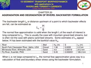
CHAPTER 17: AGGRADATION AND DEGRADATION OF RIVERS TRANSPORTING GRAVEL MIXTURES. Results of a flood in the gravel-bed Salmon River, Idaho. Photo by author. REVIEW: SEDIMENT CONSERVATION OF GRAVEL MIXTURES.

E N D
CHAPTER 17: AGGRADATION AND DEGRADATION OF RIVERS TRANSPORTING GRAVEL MIXTURES Results of a flood in the gravel-bed Salmon River, Idaho. Photo by author
REVIEW: SEDIMENT CONSERVATION OF GRAVEL MIXTURES • Gravel-bed rivers tend to be poorly-sorted. During floods, bed material load consists almost exclusively of bedload. (Sand is often transported in copious quantities as washload during floods.) The surface material (armor or pavement) tends to be coarser than the substrate. By definition the median size Dsub50 or geometric mean size Dsubg of the substrate is in the gravel range, but the substrate may contain up to 30% sand in the interstices of an otherwise clast-supported deposit. • Material from Chapters 4 and 7 is used extensively in this chapter, and is reviewed in the next few slides. Definitions follow below. • Fi = fraction of material in the surface layer in the ith grain size range, i = 1..N • Di = characteristic size of the ith grain size range • La = thickness of the surface (active, exchange) layer • fIi = fraction in the ith grain size range of material exchanged between the surface and the substrate as the bed aggrades or degrades • qbi = volume bedload transport rate per unit width of material in the ith grain size range • qbT = Sqbi = total volume bedload transport rate per unit width • pi = qbi/qbT = fraction of bedload material in the ith grain size range
REVIEW FROM CHAPTER 4: EXNER RELATIONS FOR MIXTURES The total bedload transport rate summed over all grain sizes qbT and the fraction pbi of bedload in the ith grain size range can be defined as The Exner equation of sediment conservation of Chapter 4, here generalized to include the flood intermittency If of Chapter 14, can thus be written as Summing over all grain sizes, the following equation describing the evolution of bed elevation is obtained: Between the above two relations, the following equation describing the evolution of the grain size distribution of the active layer is obtained:
REVIEW FROM CHAPTER 4: EXCHANGE FRACTIONS where 0 1 (Hoey and Ferguson, 1994; Toro-Escobar et al., 1996). In the above relations Fi, pi and fi denote fractions in the surface layer, bedload and substrate, respectively. That is: The substrate is mined as the bed degrades. A mixture of surface and bedload material is transferred to the substrate as the bed aggrades, making stratigraphy. Stratigraphy (vertical variation of the grain size distribution of the substrate) needs to be stored in memory as bed aggrades if subsequent degradation into the deposit is to be computed.
REVIEW FROM CHAPTER 7: SURFACE-BASED BEDLOAD TRANSPORT FORMULATION FOR MIXTURES Consider the bedload transport of a mixture of sizes. The thickness La of the active (surface) layer of the bed with which bedload particles exchange is given by as where Ds90 is the size in the surface (active) layer such that 90 percent of the material is finer, and na is an order-one dimensionless constant (in the range 1 ~ 2). Divide the bed material into N grain size ranges, each with characteristic size Di, and let Fi denote the fraction of material in the surface (active) layer in the ith size range. The volume bedload transport rate per unit width of sediment in the ith grain size range is denoted as qbi. The total volume bedload transport rate per unit width is denoted as qbT, and the fraction of bedload in the ith grain size range is pbi, where Now in analogy to *, q* and W*, define the dimensionless grain size specific Shields number i*, grain size specific Einstein number qi* and dimensionless grain size specific bedload transport rate Wi* as
REVIEW FROM CHAPTER 7: SURFACE-BASED BEDLOAD TRANSPORT FORMULATION contd. It is now assumed that a functional relation exists between qi* (Wi*) and i*, so that The bedload transport rate of sediment in the ith grain size range is thus given as According to this formulation, if the grain size range is not represented in the surface (active) layer, it will not be represented in the bedload transport.
REVIEW: BEDLOAD RELATION FOR MIXTURES DUE TO PARKER (1990a,b) This relation is appropriate only for the computation of gravel bedload transport rates in gravel-bed streams. In computing Wi*, Fi must be renormalized so that the sand is removed, and the remaining gravel fractions sum to unity, i.e. Fi = 1. The method is based on surface geometric size Dsg and surface arithmetic standard deviation s on the scale, both computed from the renormalized fractions Fi. In the above O and O are set functions of sgospecified in the next slide.
REVIEW: BEDLOAD RELATION FOR MIXTURES DUE TO PARKER (1990a,b) contd. o o It is not necessary to use the above chart. The calculations can be performed using the Visual Basic programs in RTe-bookAcronym1.xls
REVIEW: BEDLOAD RELATION FOR MIXTURES DUE TO WILCOCK AND CROWE (2003) The sand is not excluded in the fractions Fi used to compute Wi*. The method is based on the surface geometric mean size Dsg and fraction sand in the surface layer Fs.
MODELING AGGRADATION AND DEGRADATION IN GRAVEL-BED RIVERS CARRYING SEDIMENT MIXTURES Gravel-bed rivers tend to be steep enough to allow the use of the normal (steady, uniform) flow approximation. Here this analysis is applied using a Manning-Strickler formulation such that roughness height ks is given as where Ds90 is the size of the surface material such that 90% is finer and nk is an order-one dimensionless number (1.5 ~ 3; the work of Kamphuis, 1974 suggests a value of 2). No attempt is made here to decompose bed resistance into skin friction and form drag. The reach is divided into M intervals bounded by M + 1 nodes. In addition, sediment is introduced at a ghost node at the upstream end. Since the index “i” has been used for grain size ranges, the index “k” is used here for spatial nodes.
COMPUTATION OF BED SLOPE AND BOUNDARY SHEAR STRESS At any given time t in the calculation, the bed elevation k and surface fractions Fi,k must be known at every node k. The roughness height ks,k and thickness of the surface layer La,k are computed from the relations where nk and na are specified order-one dimensionless constants. (Beware: in the equation for roughness height the “k” in nk is not an index for spatial node.) Using the normal flow approximation, the boundary shear stress b,k at the kth node is given from Chapter 5 as where u,k denotes the shear velocity and bed slope Sk is computed as Bed slope need not be computed at k = M + 1, where bed elevation is specified as a boundary condition.
COMPUTATION OF BEDLOAD TRANSPORT Once Fi,k and b,k are known, the bedload transport rates qbi, and thus qbT and pi can be computed at any node. An example is given here in terms of the Wilcock-Crowe (2003) formulation. Using the relations of Chapter 2, the surface geometric mean size Dsg,k is calculated at every node as where i = ln2(Di). The Shields number and shear velocity based on the surface geometric mean size are then given as The same fractions Fi,k allow the computation of the fraction sand Fs,k in the surface layer at node k. This parameter is needed in the formulation of Wilcock and Crowe (2003).
COMPUTATION OF BEDLOAD TRANSPORT contd. It follows that the volume bedload transport rate per unit width in the ith grain size range is given as where in the case of the relation of Wilcock and Crowe (2003),
MODELING AGGRADATION AND DEGRADATION IN GRAVEL-BED RIVERS CARRYING SEDIMENT MIXTURES contd. The discretized versions of the Exner relations are: where fIi,k is evaluated from a relation of the type given in Slide 4: In the above relation fs,i,int,k denotes the fractions of the substrate just below the surface layer at node k and is a user-specified parameter between 0 and 1.
MODELING AGGRADATION AND DEGRADATION IN GRAVEL-BED RIVERS CARRYING SEDIMENT MIXTURES contd. The spatial derivatives of the sediment transport rates are computed as where au is a upwinding coefficient equal to 0.5 for a central difference scheme. When k = 1, the node k – 1 refers to the ghost node, where qbi, and thus qbT and pi are specified as feed parameters. The term La,k/t t is not a particularly important one, and can be approximated as where La,k,old is the value of La,k from the previous time step. In the case of the first time step, La,k,old may be set equal to 0.
BOUNDARY CONDITIONS, INITIAL CONDITIONS AND FLOW OF THE COMPUTATION • The boundary conditions are • Specified values of qb,i (and thus qbT and pbi) at the upstream ghost node; • Specified bed elevation at node k = M+1. • The initial conditions are • Specified initial bed elevations at every node (here simplified to a specified initial bed slope Sfbl; • Specified surface and substrate grain size distributions Fi and fs,i at every node (here taken to be the same at every node). • At any given time fractions Fi and elevation are known at every node. The values Fi are used to compute Ds90 Dsg, Ds50, ks, La and other parameters (e.g. Fs) at every node. The values of are used to compute slopes S and combined with the computed values of ks to determine the shear stress b at every node except M+1, where the information is not needed. The resulting parameters are used to compute qbi, qbT and pbi at all nodes except M+1. The Exner relations are then solved to determine bed elevations and surface fractions Fi at all nodes. At node M+1 only the change in grain size distribution is evaluated.
INTRODUCTION TO RTe-bookAgDegNormGravMixPW.xls The workbook is a descendant of the PASCAL code ACRONYM3 of Parker (1990a,b). It allows the user to choose from two surface-based bedload transport formulations; those of Parker (1990a) and Wilcock and Crowe (2003). In the relation of Parker (1990a) the surface grain size distributions need to be renormalized to exclude sand before specification as input to the program. This step is neither necessary nor desirable in the case of the relation of Wilcock and Crowe (2003), where the sand plays an important role in mediating the gravel bedload transport. The basic input parameters are the water discharge per unit width qw, flood intermittency If, gravel input rate during floods qbTf, reach length L, initial bed slope SfbI, number of spatial intervals M, time step t, fractions pbf,i of the gravel feed, fractions FI,i of the initial surface layer (assumed the same at every node) and fractions fsI,I of the substrate (assumed to be uniform in the vertical and the same at every node). The parameters Mprint and Mtoprint control output. Auxiliary parameters include nk for roughness height, na for active layer thickness, r of the Manning-Strickler relation, submerged specific gravity R of the sediment, bed porosity p, upwinding coefficient au and interfacial transfer coefficient .
INTRODUCTION TO RTe-bookAgDegNormGravMixPW.xls contd. One interesting problem of sediment mixtures is when the river first aggrades, creating its own substrate with a vertical structure in the process, and then degrades into it. The code in the workbook is not set up to handle this. The necessary extension is trivial in theory but tedious in practice; the vertical structure of the newly-created substrate must be stored in memory as the calculation proceeds. A gravel-bed reach of the Las Vegas Wash, USA, where the river is degrading into its own deposits. Some calculations with the code follow.
CALCULATIONS WITH RTe-bookAgDegNormGravMixPW.xls The calculations are performed with the Parker (1990a,b) bedload transport relation. The grain size distributions of the feed sediment, initial surface sediment and substrate sediment are all taken to be identical, as given below. Note that sand has been removed from the grain size distributions.
CALCULATIONS WITH RTe-bookAgDegNormGravMixPW.xls contd. A case is chosen for which the bed must aggrade from a very low slope. Calculations are performed for 60 years, 600 years and 6000 years in order to study the evolution of the profile. The software produces graphical output for the time development of the long profiles of a) bed elevation , b) surface geometric mean size Dsg and c) volume gravel bedload transport rate per unit width qbT.
Parker relation After 60 years
Parker relation After 60 years
Downstream variation of qbT/qbTf, where qbT = Bedload Transport Rate and qbTf = Upstream Bedload Feed Rate Parker relation After 60 years qbT/qbTf
Parker relation After 600 years
Parker relation After 600 years
Downstream variation of qbT/qbTf, where qbT = Bedload Transport Rate and qbTf = Upstream Bedload Feed Rate Parker relation After 600 years qbT/qbTf
Parker relation After 6000 years
Parker relation After 6000 years
Downstream variation of qbT/qbTf, where qbT = Bedload Transport Rate and qbTf = Upstream Bedload Feed Rate Parker relation After 6000 years qbT/qbTf
CALCULATIONS WITH RTe-bookAgDegNormGravMixPW.xls contd. The next case is one for which the bed which the bed must degrade to a new equilibrium. The input grain size distributions are the same as the previous case. Again, the Parker (1990a,b) relation is used. The input parameters are given below. The calculation shown is over a duration of 240 years.
Parker relation After 240 years
Parker relation After 240 years
Downstream variation of qbT/qbTf, where qbT = Bedload Transport Rate and qbTf = Upstream Bedload Feed Rate qbT/qbTf Parker relation After 240 years
CALCULATIONS WITH RTe-bookAgDegNormGravMixPW.xls contd. Sand is excluded from the input grain size distributions when using the Parker (1990a,b) relation. The Wilcock-Crowe (2003) relation explicitly includes the sand. Two calculations follow. In the first of them, the input data are exactly the same as that for the calculations using Parker (1990a,b) of Slides 30-33 (degradation to a new equilibrium). In particular, sand is excluded from the input grain size distributions. In the second of them, 25% sand is added to the grain size distribution. The Wilcock-Crowe (2003) relation predicts that the addition of sand makes the gravel more mobile. It will be seen that the bed elevation at the end of the 240-year calculation is predicted to be significantly lower when sand is included than when it is excluded.
Wilcock-Crowe relation Sand excluded After 240 years
Wilcock-Crowe relation Sand excluded After 240 years
Downstream variation of qbT/qbTf, where qbT = Bedload Transport Rate and qbTf = Upstream Bedload Feed Rate qbT/qbTf Wilcock-Crowe relation Sand excluded After 240 years
Wilcock-Crowe relation Sand included After 240 years
Wilcock-Crowe relation Sand included After 240 years
Downstream variation of qbT/qbTf, where qbT = Bedload Transport Rate and qbTf = Upstream Bedload Feed Rate qbT/qbTf Wilcock-Crowe relation Sand included After 240 years
NOTES ON THE EFFECT OF SAND IN THE GRAVEL Comparing Slides 35 and 38, it is seen that the upstream end of the reach has degraded considerably more in the case of Slide 38, i.e. when sand is included in the Wilcock-Crowe (2003) calculation. Comparing Slides 31 and 38, it is seen that the bed profile at the end of the calculation using Wilcock-Crowe (2003) with sand included is almost the same as the corresponding profile using Parker (1990a,b), in which sand is automatically excluded. The correspondence is not an accident. The field data used to develop the Parker (1990a,b) relation did indeed include sand in the bed and load; sand was excluded in the development of the relation because of uncertainty as to how much might go into suspension. So the Parker (1990a,b) relation implicitly includes a set fraction of sand in the bed. This notwithstanding, the Wilcock-Crowe (2003) relation has the considerable advantage that the quantity of sand in the feed sediment and substrate can be varied. As the calculations show, for all other factors equal the relation predicts that an increased sand content can significantly increase the mobility of the gravel.
REFERENCES FOR CHAPTER 17 Hoey, T. B., and R. I. Ferguson, 1994, “Numerical simulation of downstream fining by selective transport in gravel bed rivers: Model development and illustration,” Water Resources Research, 30, 2251-2260. Kamphuis, J. W., 1974, Determination of sand roughness for fixed beds, Journal of Hydraulic Research, 12(2): 193-202. Parker, G., 1990a, Surface-based bedload transport relation for gravel rivers,” Journal of Hydraulic Research, 28(4): 417-436. Parker, G., in press, Transport of gravel and sediment mixtures, ASCE Manual 54, Sediment Engineering, ASCE, Chapter 3, downloadable at http://cee.uiuc.edu/people/parkerg/manual_54.htm . Toro-Escobar, C. M., G. Parker and C. Paola, 1996, Transfer function for the deposition of poorly sorted gravel in response to streambed aggradation, Journal of Hydraulic Research, 34(1): 35-53. Wilcock, P. R., and Crowe, J. C., 2003, Surface-based transport model for mixed-size sediment, Journal of Hydraulic Engineering, 129(2), 120-128.