Download
1 / 62
640 likes | 810 Views
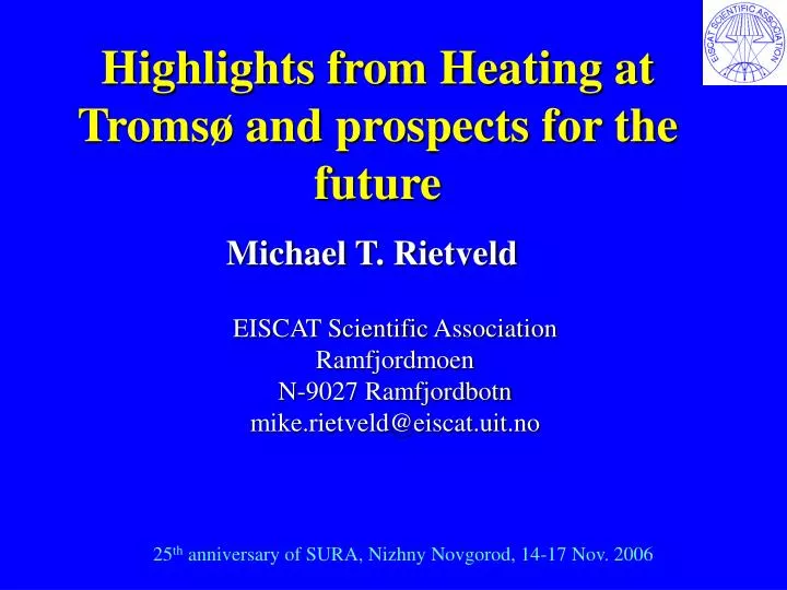
Highlights from Heating at Tromsø and prospects for the future. Michael T. Rietveld. EISCAT Scientific Association Ramfjordmoen N-9027 Ramfjordbotn mike.rietveld@eiscat.uit.no. 25 th anniversary of SURA, Nizhny Novgorod, 14-17 Nov. 2006. The Heating facility at Tromsø. Control. Antenna 1.

E N D
Highlights from Heating at Tromsø and prospects for the future Michael T. Rietveld EISCAT Scientific AssociationRamfjordmoenN-9027 Ramfjordbotnmike.rietveld@eiscat.uit.no 25th anniversary of SURA, Nizhny Novgorod, 14-17 Nov. 2006
The Heating facility at Tromsø Control Antenna 1 Transmitter Antenna 2 Antenna 3
Scientific (and operational) Highlights • 1979 First experiments with partial facility • 1979 ELF/VLF wave excitation experiments (Dowden et al., 1981)
An early example of ELF/VLF wave generation in the ionosphere using modulated HF-heating From Stubbe et al., JATP, 1982
Scientific (and operational) Highlights • 1979 First experiments with partial facility • 1979 ELF/VLF wave excitation experiments (Dowden et al., 1981) • 1981 1-m irregularity excitation in E-region (Hibberd et al., 1983)
Generation of 1-m scale irregularities in the auroral E region by O-mode HF wave pumping From Hibberd et al., JGR, 1983
Scientific (and operational) Highlights • 1979 First experiments with partial facility • 1979 ELF/VLF wave excitation experiments (Dowden et al., 1981) • 1981 1-m irregularity excitation in E-region (Hibberd et al., 1983) • 1981 SEE discovery (Thidé et al., 1982)
The first Stimulated Electromagnetic Emissions (SEE) at Tromsø From Thidé et al.., 1982
STARE backscatter (144 MHz) from the E-region (Norway radar) 4 April 2005 Tromsø
Scientific (and operational) Highlights • 1979 First experiments with partial facility • 1979 ELF/VLF wave excitation experiments (Dowden et al., 1981) • 1981 1-m irregularity excitation in E-region (Hibberd et al., 1983) • 1981 SEE discovery (Thidé et al., 1982) • 1981 Anomalous absorption, striations, thermal parametric instabilities • 1981 Langmuir turbulence measured with UHF radars (Hagfors, 1983) • 1985 Low frequency (2.7-4 MHz) array destroyed in storm • 1989 Gyroharmonic effects in SEE, AA, Te measured (Leyser et al., 1989 and many others)
Special effects appear when the HF frequency is close to a harmonic of the electron gyrofrequency (1.4 MHz). For example, artificial irregularities are weaker (upper panel) and some SEE features disappear (lower middle panel) (Honary et al., Ann. Geophys., 1999)
Gyroharmonic effects 3 Nov 2000 ERP = 70 MW O-mode UHF Cutlass Artificial aurora 630 nm Kosch et al., Geophys. Res. Lett., 29, 23, 2112, 2002
Scientific (and operational) Highlights • 1979 First experiments with partial facility • 1979 ELF/VLF wave excitation experiments (Dowden et al., 1981) • 1981 SEE discovery (Thidé et al., 1982) • 1981 1-m irregularity excitation in E-region (Hibberd et al., 1983) • 1981 Anomalous absorption, striations, thermal parametric instabilities • 1981 Langmuir turbulence measured with UHF radars (Hagfors, 1983) • 1985 Low frequency (2.7-4 MHz) array destroyed in storm • 1989 Gyroharmonic effects in SEE, AA, Te measured (Leyser et al., 1989 and many others) • 1990 Operation of the rebuilt, high-gain (30dBi) array-1 started • 1993 transfer of Heating from Max-Planck to EISCAT • 1993 First API experiment at Tromsø (Rietveld et al., 1996)
Artificial Periodic Irregularities (API) The API technique was discovered at SURA and allows any HF pump and ionosonde to probe the ionosphere. API are formed by a standing wave due to interference between the upward radiated wave and its own reflection from the ionosphere. (See book by Belikovich et al., 2001) Measured parameters include: N(n), N(e), N(O-), vertical V(i), T(n), T(i) & T(e)
An example of API decaying in two altitude ranges, one rarely observed as low as 45-65 km, the other frequently observed between 80-100 km.
Range-time-intensity plot of decaying API echoes just below and above the O-mode reflection height for two 1 s heater pulses. (Rietveld and Goncharov, Adv. Space res., 1998)
Scientific (and operational) Highlights • 1979 First experiments with partial facility • 1979 ELF/VLF wave excitation experiments (Dowden et al., 1981) • 1981 SEE discovery (Thidé et al., 1982) • 1981 1-m irregularity excitation in E-region (Hibberd et al., 1983) • 1981 Anomalous absorption, striations, thermal parametric instabilities • 1981 Langmuir turbulence measured with UHF radars (Hagfors, 1983) • 1985 Low frequency (2.7-4 MHz) array destroyed in storm • 1989 Gyroharmonic effects in SEE, AA, Te measured (Leyser et al., 1989 and many others) • 1990 Operation of the rebuilt, high-gain (30dBi) array-1 started • 1993 transfer of Heating from Max-Planck to EISCAT • 1993 First API experiment at Tromsø (Rietveld et al., 1996) • 1997 Aspect angle and other details of Langmuir turbulence (Isham et al., 1999) • 1998 Large Te increases at night, aspect-angle dependent (Rietveld et al., 2003) • 1999 Artificial aurora, magnetic zenith effect (Brändström et al., 1999, Kosch et al., 2000)
F-region plasma phenomena • In addition to having a strong dependence on the difference between HF frequency from a gyroharmonic, many phenomena show a marked dependence on the angle the HF rays make with the magnetic field (Magnetic Zenith effect) • e.g., electron heating, artificial optical emissions, Langmuir turbulence, striations, large scale irregularities. These effects remain largely unexplained.
Electron heating and UHF beam swinging UHF zenith angle 7 Oct 1999 4.954 MHz ERP = 100 MW O-mode (Rietveld et al., JGR, 2003)
Ion upwelling Electron heating HF on HF off (Rietveld et al., JGR, 2003)
decay line first cascade Cavitation spectra second cascade
PLASMA TURBULENCE 12 Nov 2001 5.423 MHz ERP = 830 MW O-mode UHF ion line spectra HF on HF off
Seeding of Langmuir turbulence by high power HF modification during aurora V. Belyey, B. Isham, T.B. Leyser and M.T. Rietveld (manuscript in preparation)
HF on HF on HF on HF on HF on HF on Plasma line Ion line 22 November 2003
HF off HF on HF off HF on Plasma line Ion line
Pump freq HF on HF off
Heater beam Spitze direction Field aligned 21 Feb 1999 6300 East=RHS South= Bottom Start time= 17.07.50 UT Step=480 sec Kosch et al.2000 Artificial aurora Airglow at 6300Å shifted from heater beam
An example of unexplained annular structures, formed by electrons accelerated through Langmuir turbulence. (Kosch et al., GRL, 2004)
The artificial auroral structure at 16:37:05 UT on12 November 2001, 5 s after HF pump turn on. Integration time =5 s. The image is taken in the zenith from Skibotn and has a 50º field of view (large circle). The -3 dB locus of the pump beam assuming free space propagation is shown as a small circle (beamwidth = 7.4º), projected at 230 km altitude and tilted 9º south of the HF facility at Ramfjordmoen. The upper cross shows the location of the HF transmitter whilst the lower cross shows the magnetic field line direction (12.8º S), both projected at 230 km. The dotted line represents the magnetic field line connected to Ramfjordmoen and the labels give altitude.(from Kosch et al., GRL, 2004)
Scientific (and operational) Highlights • 1979 First experiments with partial facility • 1979 ELF/VLF wave excitation experiments (Dowden et al., 1981) • 1981 SEE discovery (Thidé et al., 1982) • 1981 1-m irregularity excitation in E-region (Hibberd et al., 1983) • 1981 Anomalous absorption, striations, thermal parametric instabilities • 1981 Langmuir turbulence measured with UHF radars (Hagfors, 1983) • 1985 Low frequency (2.7-4 MHz) array destroyed in storm • 1989 Gyroharmonic effects in SEE, AA, Te measured (Leyser et al., 1989 and many others) • 1990 Operation of the rebuilt, high-gain (30dBi) array-1 started • 1993 transfer of Heating from Max-Planck to EISCAT • 1993 First API experiment at Tromsø (Rietveld et al., 1996) • 1997 Aspect angle and other details of Langmuir turbulence (Isham et al., 1999) • 1998 Large Te increases at night, aspect-angle dependent (Rietveld et al., 2003) • 1999 Artificial aurora, magnetic zenith effect (Brändström et al., 1999, Kosch et al., 2000) • 1998 ULF waves and Ionopsheric Alfven Resonator (Robinson et al., 2000)
Ultra Low Frequency waves (3 Hz) Field line tagging
A schematic of the artificial 3-Hz ULF wave injection from the ionospheric source region, along the geomagnetic field line, beyond the spacecraft to the Ionospheric Alfvén Resonator boundary at about 1.5 RE. Here the wave acquires a significant electric field component parallel to the geomagnetic field and can accelerate electrons down past the spacecraft toward the ionosphere, as well as away from the spacecraft, out into space. (After Wright et al., J. Geophys. Res., 2003)
Scientific (and operational) Highlights • 1979 First experiments with partial facility • 1979 ELF/VLF wave excitation experiments (Dowden et al., 1981) • 1981 SEE discovery (Thidé et al., 1982) • 1981 1-m irregularity excitation in E-region (Hibberd et al., 1983) • 1981 Anomalous absorption, striations, thermal parametric instabilities • 1981 Langmuir turbulence measured with UHF radars (Hagfors, 1983) • 1985 Low frequency (2.7-4 MHz) array destroyed in storm • 1989 Gyroharmonic effects in SEE, AA, Te measured (Leyser et al., 1989 and many others) • 1990 Operation of the rebuilt, high-gain (30dBi) array-1 started • 1993 transfer of Heating from Max-Planck to EISCAT • 1993 First API experiment at Tromsø (Rietveld et al., 1996) • 1997 Aspect angle and other details of Langmuir turbulence (Isham et al., 1999) • 1998 Large Te increases at night, aspect-angle dependent (Rietveld et al., 2003) • 1999 Artificial aurora, magnetic zenith effect (Brändström et al., 1999, Kosch et al., 2000) • 1998 ULF waves and Ionopsheric Alfven Resonator (Robinson et al., 2000) • 1999 PMSE modification (Chilson et al., 2000) • 2003 PMSE overshoot (Havnes et al., 2003)
Ionospheric and atmospheric physics from Heating Although plasma physics research remains an interesting and important goal of HF-ionosphere interactions, using the HF facility to learn about the atmosphere, ionosphere and magnetosphere is becoming increasingly important, as the next example shows.
Universal Time (hours) Polar Mesospheric Summer Echoes (PMSE)
How does HF affect PMSE ? • 1) PMSE weakening • HF wave heats the electrons from about 150K to some hundreds K • Heated electrons means density fluctuations smoothed out (increased diffusion). So PMSE weakens with HF on, and returns immediately with HF off. • 2) PMSE Overshoot • Dust (> 1nm particles) have electrons attached. The dust charging and electron gradients depend on particle size and density, electron density and electron temperature. The time constant to discharge to undisturbed state during off is long. • Useful diagnostic of dusty plasma since small particles charge slowly and large particles charge quickly.
How does HF affect PMSE ? 1) PMSE weakening VHF radar Artificial HF modulation of Polar Mesospheric Summer Echoes. VHF backscatter power reduces by >40 dB. Reduction occurs on timescales less than 30 ms. 10 July 1999 5.423 MHz ERP = 630 MW X-mode HF 10s ON, 10s OFF HF off HF on (Chilson et al., GRL, 2000)
Interpretation (see Rapp and Lübken, GRL, 2000) • Increasing electron temperature compensates the effect of negatively charged aerosols on the diffusion of electrons. Increasing Te enhances electron diffusion and destroys PMSE. In terms of the Schmidt number, Sc, which is the ratio of kinematic viscosity to the effective diffusion coefficient of the electrons, Sc = /Deeff is reduced. Without aerosols Sc 1. • This is the first direct experimental proof that it is indeed the reduction ofelectron diffusion by charged aerosols which allows for theexistence of scattering structures in the electron gas at very small scales. • Using the particle charging model of Rapp and Lübken [2000] we find that an electron temperature increase also leads to an enhanced charging of the aerosols. Some of the aerosol particles acquire a second or even a third electron while for "normal" electron temperatures they are singly negatively charged. This implies that the total number of charges on the aerosol increases with increasing electron temperature. Increasing the aerosol charge, however, should support PMSE [Cho et al., 1992] al. Therefore this effect is minor. • This experimental result doesnothelp solve the real problem of PMSE, namely how can structures with these sizes exist in the aerosol gas.
Smoothed data Total PMSE intensity (sum of highest intensities at each time sample) Raw data 2) PMSE overshootimmediately after switching the 3s long heater pulse off. The background noise on this linear scale is at approximately 2500. (Havnes et al., GRL, 2003.)
Model calculations showing how the shape of the overshoot phenomenon depends on particle size. HF is on from 20 to 40 s. The amplitude from 0 to 1 depends on the electron heating. (Havnes et al., GRL, 2003)
Polar Mesospheric Winter Echoes (PMWE) • Weaker than PMSE • Lower altitude than PMSE • Not associated with NLC • Not during extreme cooling No consensus yet on the several mechanisms advanced: Charged dust, Viscosity waves from breaking Infra-sonic waves. Heating effects may decide.
”First observations of the artificial modulation of Polar Mesospheric Winter Echoes” A.J. Kavanagh, F. Honary, M. T. Rietveld and A. Senior.(Geophys. Res. Lett., 33, 2006)
HF ON HF-supression of PMWEKavanagh et al., 2006 (Geophys. Res.Lett, 33, 2006)
Scientific (and operational) Highlights • 1979 First experiments with partial facility • 1979 ELF/VLF wave excitation experiments (Dowden et al., 1981) • 1981 SEE discovery (Thidé et al., 1982) • 1981 1-m irregularity excitation in E-region (Hibberd et al., 1983) • 1981 Anomalous absorption, striations, thermal parametric instabilities • 1981 Langmuir turbulence measured with UHF radars (Hagfors, 1983) • 1985 Low frequency (2.7-4 MHz) array destroyed in storm • 1989 Gyroharmonic effects in SEE, AA, Te measured (Leyser et al., 1989 and many others) • 1990 Operation of the rebuilt, high-gain (30dBi) array-1 started • 1993 transfer of Heating from Max-Planck to EISCAT • 1993 First API experiment at Tromsø (Rietveld et al., 1996) • 1997 Aspect angle and other details of Langmuir turbulence (Isham et al., 1999) • 1998 Large Te increases at night, aspect-angle dependent (Rietveld et al., 2003) • 1999 Artificial aurora, magnetic zenith effect (Brändström et al., 1999, Kosch et al., 2000) • 1998 ULF waves and Ionopsheric Alfven Resonator (Robinson et al., 2000) • 1999 PMSE modification (Chilson et al., 2000) • 2003 PMSE overshoot (Havnes et al., 2003) • 2004 Interferometry of SEE (Isham et al., 2005; Tereshchenko et al., 2006)
SEE interferometer data from 5 October 2004 at EISCAT on Ramfjordmoen showing anexpanded view of thefrequency scale encompassing the BUM1, and showing thecoherences for all three antenna baselines plus elevationand azimuth angles computed for the BUM1 source region. The elevation angle of the BUM1 is about 74 deg during the pump cycle beginningat 10:56 UT and about 70 during the follow two cycles. The HF beam was centred on 14 deg south for the first and 17.5 deg S for the next two cycles. Time and frequency resolutions are 1 s and 1 kHz. From Isham et al., Ann Geophys., 2005
SEE interferometer data from 5 October 2004 at EISCAT on Ramfjordmoen. A view of the portion of the frequency scale encompassing the DM, and showing the power spectrum, the coherences for all threeantenna baselines, plus elevation and azimuth angles computed for the DM source region. The DM can be seen between about -10 and-12 kHz relative to the pump frequency. The elevation angle of the DM is about 77 deg during the pump cycle beginning at 10:56 UT and about73 deg during the follow two cycles. Time and frequency resolutions are 1 s and 200Hz From Isham et al., Ann Geophys., 2005
Cross power (unnormalized coherence) curves calculated from raw voltage samples from the pairs of the north–south receiver channels (the left panels) and west–east receiver channels (the right panels). The top row of spectra were made using a noise generator and the 4040-kHz notch filters connected to each receiver. The bottom panels show the corresponding experimental SEE cross power spectra, measured 6.5 min after the pump on time at 15:30 UT on 6 October 2004, using the 4040-kHz notch filters with the pump transmitting at 4040 kHz. The vertical line is plotted at 4038.8 kHz, slightly below the filter cutoff frequency. From Tereshchenko et al., Ann Geophys., 2006
SEE power spectral densities for the north (left column), south (central column), and west (right column) antennas at four different times and antenna beam directions. Both the DP component and the narrow continuum (NC) are clearly seen in the SEE spectra. The time at the left of each plot refers to minutes after 15:30 UT on 6 Oct 2004. The beam direction is degrees south of vertical. From Tereshchenko et al., Ann Geophys., 2006