Download
1 / 46
490 likes | 749 Views
Chapter 4 Simplex Method for Linear Programming. Shi-Shang Jang Chemical Engineering Department National Tsing-Hua University. Example 1: Inspector Problem.

E N D
Chapter 4 Simplex Method for Linear Programming Shi-Shang Jang Chemical Engineering Department National Tsing-Hua University
Example 1: Inspector Problem • Assume that it is desired to hire some inspectors for monitoring a production line. A total amount of 1800 species of products are manufactured every day (8 working hours), while two grades of inspectors can be found. Maximum, 8 grade A inspector and 10 grade B inspector are available from the job market. Grade A inspectors can check 25 species/hour, with an accuracy of 98 percent. Grade B inspectors can check 15 species/hour, with an accuracy of 95 percent. Note that each error costs $2.00/piece. The wage of a grade A inspector is $4.00/hour, and the wage of a grade B inspector is $3.00/hour. What is the optimum policy for hiring the inspectors?
Problem Formulation • Assume that the x1grade A inspectors x2 grade B inspects are hired, then • total cost to be minimized • 48x1+38 x2+2580.022x1+1580.052x2 =40 x1+36 x2 • manufacturing constraint • 258x1+158x21,800 200 x1+120 x21,800 • no. of inspectors available: • 0 x18 • 0 x210
Theorem • Property: If there exists an optimal solution to a LP, then at least one of the corner point of the feasible region will always qualify to be an optimal solution.
Special Cases • Alternate Solutions (non-unique solutions) • Max x1+2x2 • s.t. x1+2x210 • x1+ x21 • x24 • x10, x20
Special Cases - continued • Unbounded Optima : A system has a feasible region with open boundaries such that the optima may appear at the infinity. • Example: For the previous example, in case the constraint x1+2x210 is not given, then moving far away from the origin increases the objective function x1+2x2, and the maxim Z would be +
Unbounded Optima x2=4 x1+2x2=15 x1+2x2=10 x1+2x2=6 x1+2x2=2 x1+x2=1
Example 2: Student Fab • The RIT student-run microelectronic fabrication facility is taking orders for four indigenously developed ASIC chips that can be used in (1) touch sensors ($6, s4hr, m1hr, v30), (2)LCD($10,s9hr, m1hr, v40), (3) pressure sensors($9, s7hr, m3hr, v20), and (4) controllers($20, s10hr, m8hr, v10). • Constraints : Student hr≦ 600, machine hr≦420, space≦800
4-2 The Basic Approach • Standard Form of Linear Programming
Handling of in-equality Constraints • Case 1: Slack Variable: x1+2x2+3 x3+4x425 • Modified to x1+2x2+3x3+4x4+ x5=25 x50 is a slack variable. • Case 2: Surplus Variable: 2 x1+ x2-3 x312 • Modified to 2 x1+ x2-3 x3- x4=12 x40 is a surplus variable.
Handling of Equality Constraints • If s is unrestricted, i.e., s can be positive or negative, then we set • s=s+-s- • such that s+0, s-0.
Example Modify to
Definitions • Definition: A feasible region, denoted by S is the set of all feasible solution. Mathematically, . • Definition: An optimal solution is a vector x*S, s.t. z0=cTx* is maximum or minimum in where Z is termed by the optimal value. • Definition: Alternate optimal solution is a set XS, s.t. all xX has the same objective value z0 and for all xS, and z=cTx, z z0. • Definition: If the solution set of LP contains only one element, it is termed the unique optimum. • Definition: If the optimum value z approaches to infinity, then the LP is said to have unbounded optimum.
Definitions • Definition: A pivot operation is sequence of elementary row operations that reduce the coefficients of a specified variable to unity in one of the equation and zero elsewhere. • Definition: In the above canonical form, x1,,xm are termed the basic variables or dependent variables, xm+1, ,xn are called nonbasic variables or the independent variables. • Definition: The solution obtained from a canonical form is by setting the nonbasic variable or independent variable to zero is called a basic solution. • Definition: A basic feasible solution is a basic solution in which the basic or dependent variables are non-negative.
Property Remark: where Definition: Property: A feasible basic solution is a simplex of the feasible region. Note: Given a canonical form and feasible basic solution, then the objective function: where xB is a basic variable.
Approach (Simplex Method): • Start with an initial basic feasible solution in canonical form. • Improve the solution by finding another basic feasible solution if possible. • When a particular basic feasible solution is found, and cannot be improved by finding new basic feasible solution, the optimality is reached. • Definition: An adjacent basic solution differs from a basic solution is exactly one basic variable. • Question: If one wants to find an adjacent feasible basic solution from one feasible basic solution (i.e., switch to another simplex), which adjacent basic solution gives lowest objective function?
Derivation of Inner Product Rule Supposing, one wants to replace one of the original basic variable with nonbasic variable xs, we firstly, increase xs from zero to one, then for all i=1,,m, and, for all j=m+1, ,n, js. xj=0
Theorem 1 (Inner Product Rule) Relative cost, (inner product rule) More: (1) In a minimization problem, a basic feasible solution is optimal if the relative costs of its all nonbasic variable are all positive or zero. (2) One should choose an adjacent basic solution from which the relative cost is the minimum. Corollary: The alternate optima exists if z=0.
Theorem 2: (The Minimum Ratio Rule ) • Given a nonbasic variable xs is change into the basic variable set, then one of the basic variable xr should leave from the basic variable set, such that: The above minimum happens at i=r. Corollary: The above rule fails if there exist unbounded optima.
Example: Multi-Products Manufacturing • A company manufactures three products: A, B, and C. Each unit of product A requires 1 hr of engineering service, 10 hr of direct labor, and 3lb of material. To produce one unit of product B requires 2hr of engineering, 4hr of direct labor, and 2lb of material. In case of product C, it requires 1hr of engineering, 5hr of direct labor, and 1lb of material. There are 100 hr of engineering, 700 hr of labor, and 400 lb of material available. Since the company offers discounts for bulk purchases, the profit figures are as shown in the next slide:
Example- Continued Formulate a linear program to determine the most profitable product mix.
Problem Formulation Let’s denote the variables as shown in the table, then we have the following:
MATLAB PROGRAM • f=[-10 -9 -8 -7 -6 -4 -3 -5 -4]'; • A=[1 1 1 1 2 2 2 1 1; 10 10 10 10 4 4 4 5 5;3 3 3 3 2 2 2 1 1]; • b=[100;700;400]; • Aeq=[];beq=[]; • LB=[0 0 0 0 0 0 0 0 0]; • UB=[40 60 50 Inf 50 50 Inf 100 Inf]; • [X,FVAL,EXITFLAG,OUTPUT,LAMBDA]=LINPROG(f,A,b,Aeq,beq,LB,UB)
Solution • X’= 40.0000 22.5000 0.0000 0.0000 18.7500 0.0000 0.0000 0.0000 0.0000 • FVAL =-715.0000 • EXITFLAG =1 • OUTPUT = • iterations: 7 • cgiterations: 0 • algorithm: 'lipsol' • LAMBDA = • ineqlin: [3x1 double] • eqlin: [0x1 double] • upper: [9x1 double] • lower: [9x1 double]
3. Sensitivity Analysis • Shadow Prices: To evaluate net impact in the maximum profit if additional units of certain resources can be obtained. • Opportunity Costs: To measure the negative impact of producing some products that are zero at the optimum. • The range on the objective function coefficients and the range on the RHS row.
Example • A factory manufactures three products, which require three resources – labor, materials and administration. The unit profits on these products are $10, $6 and $4 respectively. There are 100 hr of labor, 600 lb of material, and 300hr of administration available per day. In order to determine the optimal product mix, the following LP model is formulated and solve:
Optimal Solution and Sensitivity Analysis • x1=33.33, x2=66.67,x3=0,Z=733.33 • Shadow prices for row 1=3.33, row 2=0.67, row 3=0 • Opportunity Costs for x3=2.67 • Ranges on the objective function coefficients: 6≦c1(10)≦15, 4≦c2(6)≦10, -∞≦c3(4)≦6.67
Optimal Solution and Sensitivity Analysis- Continued • 60≦b1(100)≦150, 400≦b2(600)≦1000, 200≦b3(300)≦∞
100% Rules • 100% rule for objective function coefficients • 100% rule for RHS constants
Examples • Unit profit on product 1 decrease by $1, but increases by $1 for products 2 and 3, will the optimum change?(δc1=-1, Δc1=-4, δc2=1, Δc2=4, δc3=1, Δc3=2.67) • Simultaneous variation of 10 hr decrease on labor 100 lb increase in material and 50hr decrease on administration