Download
1 / 63
640 likes | 649 Views
SOLVING LINEAR PROGRAMMING PROBLEMS: The Simplex Method. Simplex Method. Used for solving LP problems will be presented Put into the form of a table, and then a number of mathematical steps are performed on the table

E N D
SOLVING LINEAR PROGRAMMING PROBLEMS: The Simplex Method
Simplex Method • Used for solving LP problems will be presented • Put into the form of a table, and then a number of mathematical steps are performed on the table • Moves from one extreme point on the solution boundary to another until the best one is found, and then it stops • A lengthy and tedious process but computer software programs are now used easily instead • Programs do not provide an in-depth understanding of how those solutions are derived • Can greatly enhance one's understanding of LP
First Step • First step is to convert model into standard form • s1 and s2, represent amount of unused labor and wood • No chairs and tables are produced, s1=40 and s2=120 • Unused resources contribute nothing to profit, Z=0 • Decision variables as well as profit at origin are:
Assigning (n-m) Variables Equal to Zero • Determine values of variables at every possible solution point • Have two equations and four unknowns, which makes direct simultaneous solution impossible • Assigns n-m variables=0 • n=number of variables • m=number of constraints • Have n = 4 variables and m = 2 constraints • x1 = 0 and s1 = 0 and substituting them results in x2 = 20 and s2=60
Feasible and Basic Feasible Solution • Solution corresponds to A • Referred to as a basic feasible solution • Feasible solution is any solution that satisfies the constraints • Basic feasible solution not only satisfies the constraints but also contains as many variables with nonnegative values as there are model constraints • m variables with nonnegative values and n-m values equal to zero X1=0 chairs S1=0 X2=20 tables S2=60 A B C
Feasible and Basic Feasible Solution • x2=0 and s2=0, results in x1=30 and s1=10 • Corresponds to point C • s1=0 and s2=0, results in two equations with two unknown variables • Get a solution which corresponds to point B, where x1=24, x2=8, s1=0, and s2= 0 • Previously identified as optimal solution point A X1=30 chairs S1=10 X2=0 tables S2=0 B C
Two Questions • Two questions can be raised by the identification of solutions at points O, A, B, and C • How was it known which variables to set equal to zero? • How is the optimal solution identified? • Answers these questions by performing a set of mathematical steps • Determines at each step which variables should equal zero and when an optimal solution has been reached X1=0 chairs S1=0 X2=20 tables S2=60 A X1=24 chairs S1=0 X2=8 tables S2=0 B X1=30 chairs S1=10 X2=0 tables S2=0 C
Initial Tableau • Model is put into the form of a table, or tableau • Our maximization model • Z = 40x1 + 50x2 + 0s1 + 0s2 Subject to x1 + 2x2+ s1 = 40 4x1 + 3x2 + s2 =120 x1, x2 , s1, s2≥ 0 • Initial simplex tableau with various column and row headings • Record the model decision variables, followed by the slack variables • Bottom rows represent constraint equations whose right-hand sides are given in the “solution” column • z-row is obtained from z -40x1-50x2=0
Determining Basic Feasible Solution • Determine a basic feasible solution • Know which two variables will form the basic feasible solution and which will be assigned a value of zero? • Selects the origin as the initial basic feasible solution • x1= 0 and x2= 0; variables in basic feasible solution are s1 and s2 which are listed under column "Basic" and their values, 40 and 120, are listed under column “solution“ • Z=0 under column “solution”
Entering Variable • Interested in giving us either some chairs or some tables • Want nonbasic variables will enter solution and become basic • z-row values represent increase per unit of entering a nonbasic variable into the basic solution • Make as much money as possible • Select variable x2 as the entering basic variable • has the greatest increase in profit per unit, $50—the most negative value in the z-row • x2 column is highlighted and is referred to as the pivot column • Referred to in mathematical terminology as pivot operations
Entering Variable by Graphical Solution • Demonstrated by the graph • At the origin nothing is produced • Moves from one solution point to an adjacent point • Move along either the x1 axis or the x2 axis • Chooses x2 as the entering variable X1=0 chairs X2=20 tables A X1=24 chairs X2=8 tables B X1=30 chairs X2=0 tables O C
Leaving Basic Variable R • One of s1 or s2 has to leave and become zero • Produce tables as many as possible • Check availability of our resources • Using labor constraint, maximum we can produce table is 20 • Enough labor is available to produce 20 tables • Using wood, maximum we can produce is 40 • Limited to 20 tables • Point A is feasible, whereas point R is infeasible Wood constraint A Labor constraint B C
Leaving Variable • Determined by dividing RHS values by pivot column values • Leaving basic variable is variable with minimum nonnegative ratio • s1 is leaving variable • s1 row is referred to as pivot row • Value of 2 is called pivot number or pivot element • Entering variable, x2, in the new solution also equals 20 • Z also increases from 0 to 1000
Second Tableau • Nonbasic and basic variables at solution point Nonbasic: x1 and s1 Basic: x2 and s2 • Various values are computed using pivot row and all other rows • First, x2 row, is computed by using every value in pivot row of first (old) tableau and divide it by pivot number, or (0/2 1/2 2/2 1/2 0/2 40/2) • New row values are shown in Table
0-(3)*0=0 4-(3)*1/2=-5/2 3-(3)*1=0 0-(3)*1/2=--3/2 1-(3)*0=1 120-(3)*20=60 1-(-50)*0=1 -40-(-50)*1/2=--15 -50-(-50)*1=0 0-(-50)*1/2=25 0-(-50)*0=0 0-(-50)*20=1000 Second Tableau-Cont. • For the remaining row values, use New row=(current row)-(its pivot column coefficient) x (New pivot row) • Requires use of both old tableau and new one • Various values for new z-row and s2-row: Z-row= current z-row – (-50)x new pivot row S2-row=current s2-row – (3)x new pivot row • Values are inserted in Table
Checking Optimal Solution • Set nonbasic variables x1 and s1 to zero, solution column provides new basic solution x2=20, s2=60 and z=1000 • Is not optimal • x1 has a negative coefficient • Select variable x1 as entering basic variable • Ratio computations, show that s2 is the leaving variable • Steps are repeated to develop the third tableau • Pivot row, pivot column, and pivot number are indicated in Table
Third Tableau • New pivot row, x1, is computed using the same formula • All old pivot row values are divided by 5/2 • Values for z-row and s2-row are computed here and shown in Table
Checking Optimal Solution • Coefficient of nonbasic variables are positive • Optimal solution has been reached • x1 = 24 chairs, x2= 8 tables and z= $1,360 profit • Corresponds to point B shown previously
Summary of the Simplex • Transform constraint inequalities into equations • Set up the initial tableau • Determine the pivot column (entering nonbasic solution variable) • Determine the pivot row (leaving basic solution variable) • Compute the new pivot row values • Compute all other row values • Determine whether or not the new solution is optimal • If these coefficients are zero or positive, the solution is optimal • If a negative value exists, return to step 3 and repeat the simplex steps
Simplex Tableaus by TORA • Used manually to solve relatively small problems • Can be so time-consuming and subject to error that manual computation • Computer solution has become so important • Many computer programs use the simplex method • Computer output includes option to display simplex tableaus • Simplex tableaus provided by TORA software
Minimization Problem • Demonstrated simplex method for a maximization problem • A minimization problem requires a few changes • Recall the minimization model minimize Z = 6 x1 + 3 x2 subject to 2 x1 + 4 x2≥ 16 4 x1 + 3 x2≥ 24 x1 and x2≥ 0 • Transformed this model into standard form by subtracting surplus variables 2 x1 + 4 x2 – s1 = 16 4 x1 + 3 x2 – s2 = 24
Introducing Artificial Variable A • Simplex method requires initial basic solution at the origin • Test this solution at origin • Violates the non-negativity restriction • Reason is shown in Figure • Solution at origin is outside feasible solution space • Add an artificial variable (R1) to the constraint equation • Create an artificial positive solution at the origin • Artificial solution helps get the simplex process started • Not want it to end up in the optimal solution • Our phosphate constraint becomes 2 x1 + 4 x2 – s1 + R1= 16 Feasible area B C
Effect of Surplus and Artificial Variables on Objective Function • Effect of surplus and artificial variables on objective function • Surplus variable has no effect on objective function • 0 is assigned to each surplus variable • Must also ensure that an artificial variable is not in the final solution • Achieved by assigning a very large cost • Assign a value of M, which represents a large positive cost • Produces objective function: • Minimization model can now be summarized as minimize Z = 6 x1 + 3 x2 + MR1 + MR2 subject to 2 x1 + 4 x2 – s1 + R1 = 16 4 x1 + 3 x2 – s2 + R2 = 24 x1, x2, s1, s2, R1, R2≥ 0.
Initial Tableau • Developed in the same way • Use R1 and R2 as a starting basic solution • x1=x2=s1=s2=0 and R1=16 and R2=24 • Notice that the origin is not in the feasible solution area • Artificially created solution • Simplex process moves toward feasibility in subsequent tableaus • Decision variables are listed first, then surplus variables, and finally artificial variables • z=24xM+16xM=40M instead of 0 • Explained in the subsequent slides
Modification in Initial Tableau • Inconsistency exists because R1 and R2 coefficient have nonzero coefficient • Eliminate this inconsistency by substituting out R1 and R2 in the z-row • We can write R1 =16-2 x1 -4 x2 +s1 R2 = 24-4 x1 -3 x2 + s2 • Substituting R1 and R2 in objective function Z = 6 x1 + 3 x2 + M (16-2 x1 -4 x2 +s1 )+ M(24-4 x1 -3 x2 + s2 ) Z = 40M+x1 ( 6-6M)+x2 (3-7M) +Ms1+ Ms2 • Transforming objective function into standard form Z +x1 ( -6+6M)+x2 (-3+7M)-Ms1- Ms2= 40M • Must be used as the z-row
Entering and Leaving Variables • Modified tableau thus becomes • z=40M, which is consistent now with values of the starting basic feasible solution R1=24 and R2=16 • x2 column is selected as the entering variable because 7M - 3 is the largest value in z-row • R1 is selected as leaving basic variable because the ratio of 4 • Second tableau is developed using simplex formulas
Second Tableau • Second tableau is shown in Table • R1 row has been eliminated • Once an artificial variable leaves basic feasible • Will never return
Third Tableau • Third tableau starts replacing R2 with x1 • R1 and R2 rows have been now eliminated • x1 row was selected as the pivot row • -4 value for the x2 row was not considered
Forth Tableau (Optimal Solution) • Starts replacing s1 with x1 • Turns out into final tableau which gives optimal solution • z-row contains no positive values • Optimal solution: • x1=0, s1=16, x2=8, s2= 0, and Z = $24
Mixed Constraints LP Problems • Discussed maximization problems with all “≥” constraints and minimization problems with all “≤” constraints • Solve a problem with a mixture of “≤”, “≥”, and “=“ constraints • A maximization problem with “≤”, “≥”, and “=“ constraints Max z=$400x1+200x2 Subject to x1+x2=30 2x1+8x2≥80 x1≤20 x1, x2≥0
First Step • Transform the inequalities into equations • First constraint is an equation • Not necessary to add a slack variable • Test it at the origin • Constraint is not feasible in this form • “≥” constraint did not work at origin either • Same thing can be done here • At the origin, x1=0 and x2=0,0 + 0 + R1= 30; R1=30 • Artificial variable cannot be assigned a positive value of M in objective function • A positive M value would definitely end up in final solution • Must give artificial variable a large negative value, or —M • Other constraints are transformed into equations • Completely transformed LP problem Max z=$400x1+200x2-MR1-MR2 s.t. x1+x2+R1=30 2x1+8x2-s1+R2=80 x1+s2=20
Initial Tableau • Initial tableau is shown in Table • Basic solution variables are a mix of artificial and slack variables • Second, third, and optimal tableaus are shown in following slides
Optimal Tableau • Solution is: x1=20, x2=10, s1=40 Z=10,000
Transforming Rules • Rules for transforming all three types of model constraints • Are as follows
Simplex Method of the 2nd Example • Steps: • Starts at origin, point A • Moves to an adjacent corner point, either B or F • Because of higher coefficient of x1, it moves toward corner point B • At B, the process is repeated for higher z value • Finds point C (the final one) • Three iterations E D C F A B Max z=3x1+2x2 s.t. x1 +2x26 2x1+x2 8 -x1+x2 1 x2 2 x1, x20 A B C
Basic and Nonbasic Variables • Basic and nonbasic variables associated with two points A and B • At point B, s2 enters as a nonbasic variable and x1 leaves as a basic variable A B
The Standard Form and the General Concept Max z=3x1 +2x2+0s1 +0s2 +0s3 +0s4 s.t. x1 +2x2+s1 =6 2x1 +x2 +s2 =8 -x1 +x2 +s3 =1 x2 +s4=2 x1,x2,s1,s2,s3,s40 • m equations (m=4) • n unknowns (n=6) • Sets (n-m) variables to zero and then solves for the remaining m unknowns • The variables set equal to zero are called nonbasic variables. The remaining ones are called basic variables • At point A, x1 =x2=0 which yields s1 =6, s2 =8, s3=1, and s4=2 • At point B, s2 =x2=0, which yields x1 =4, s1 =2, s3=5, and s4=2 A B
The Simplex Method in Tabular Form z-3x1 -2x2+0s1 +0s2 +0s3 +0 s4 =0 Obj fcn x1 +2x2+s1 =6 2x1 +x2 +s2 =8 -x1 +x2 +s3 =1 x2 +s4 =2 Constraint Equations
Initial Tableau • The basic column identifies the current basic variables s1, s2, s3, and s4 • The nonbasic variables x1 and x2 are not present in the basic column and are equal to zero • The value of Obj Fcn is z=3*0+2*0+6*0+8*0+1*0+2*0=0
Example: • The column associated with the entering variable is called entering column • The row associated with leaving variable is called pivot equation • The element at the intersection of the entering column and pivot row is called pivot element 2
Complete New Tableau • x1 =4, x2=0, and z=12 (point B) • Nonbasic variables: x2 and s2 (zero variables) • Basic variables: s1, x1, s3, and s4 • (nonzero variables) • x2 enters the solution • s1 leaves the solution • The obj fcn can be improved by 4/3*1/2=2/3 3/2
Iteration 3-Optimal New pivot s1-Equation=old s1-Equation /1.5 New z-Equation=old z-Equation – (-1/2) *new pivot equation New x1 -Equation=old x1 -Equation – (1/2) * new pivot equation New s3 -Equation=old s3 -Equation – (3/2) * new pivot equation New s4 -Equation=old s4-Equation – (1) * new pivot equation x1 =4/3, x2=10/3, and z=38/3 (point C)
Interpreting the Simplex Tableau • The optimum solution • The status of the resources • The unit worth of the resources • The sensitivity of the optimum solution to changes in the availability of resources, coefficients of the obj fcn, and usage of resources by activities • The first three are in optimal solution of the simplex tableau • Forth one needs additional computations
Summary • Simplex method was introduced as algebraic procedure for solving LP problems • Described how initial tableau of a linear program is a necessary step in the simplex solution procedure, including (≤), (≥), and (=) constraints into tableau form • Discussed how the special cases of infeasibility, unboundedness, multiple optimal solution, and degeneracy can occur with the simplex method
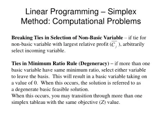
Special Cases in the Simplex Method • Special types of LP problems need special attentions • Special types: • More than one optimal solution • Infeasible problems • Unbounded solutions • Ties for pivot column and/or ties for the pivot row • Constraints with negative quantity values